# load tidyverse:
library(tidyverse)

# load data:
chi_tea <- readr::read_csv("data/tea_position.csv") Tutorial 07: Chi-square
In Hot Water
You may remember this horrific abomination interesting interpretation of the tea-making process that blew up a couple years ago. Many people, including my (Jennifer’s) English partner1, were thoroughly scandalised, but it raises an interesting question: does changing the order of the steps actually change the taste?
Here’s the video in question, if you would like a nice steaming cup of absolute outrage.
Americans making hot tea 🍵 #americanintheuk @mleemaster10
You may know someone - or be that someone yourself! - who is convinced that you can tell the difference when someone makes tea “wrong”. Well, whether there is a right or wrong way to make a cuppa is a matter of opinion2, but whether someone can accurately identify a difference in taste is a matter of science. So - let’s design an experiment and then analyse the data to find out!
A Lady Tasting Tea
This particular research question is very appropriate for our statistical test today. In 1935, botanist Dr Blanche Muriel Bristol claimed that she could tell whether the milk had been added before or after the tea. Her claim was apparently substantiated by her subsequent performance on eight randomly presented cups of tea, four with the milk first and four with the tea first. The person testing her on this claim was dapper young scientist, future founding father of statistical analysis, and resolute eugenicist Ronald Fisher, who subsequently described a version of this experiment in the 1935 paper “A Lady Tasting Tea”. This paper set out Fisher’s idea of the null hypothesis for the first time.
Data and Design
Our experiment today will be based on this excellent investigation by students at the University of Sheffield, which includes full descriptions of the results and instructions for doing your own tea taste test with your family, friends, or flatmates. In case you’re not up for making a few hundred cups of tea in the name of Science, we’ll use that study’s data instead, graciously provided by Dr Tom Stafford.
Task 1
Load packages and read data
- Load the tidyverse package
- Read in the data stored in
data/tea_position.csv. I’ve called minechi_tea, but you do you.
- Have a poke around this dataset to get familiar with it. How many participants were there in this experiment? How many variables? What are the variables called?
Hint
There are many ways to check information about datasets. Some functions are covered in the tutorial on summarising data. You can also write the name of the dataset into the codechunk to display it - most of the info will be visible this way.
Solution
# number of participants:
nrow(chi_tea)
[1] 95# number of variables
ncol(chi_tea)[1] 3# variable names
names(chi_tea)[1] "believe_position" "actual_position" "correct" # overall summary
summary(chi_tea) believe_position actual_position correct
Length:95 Length:95 Length:95
Class :character Class :character Class :character
Mode :character Mode :character Mode :character As we discussed in the lecture, a test of association (also called a test of independence) investigates whether two variables are associated with each other. In this case, we want to know whether there is an association between the location of the milk-first cup of tea (left or right), and the participant’s belief about the location of the milk-first cup of tea (left or right).
Task 2
Stop and think about this design before we go on
- What are the null and alternative hypotheses?
- What pattern would we expect to see in the data in each of these cases?
- What do you predict the result will be - do you think that people will be able to correctly identify the milk-first tea? Do you think you could?
- Write down your thoughts in the notebook document.
Solution
An example of a null hypothesis is “There will be no association between the actual position and participants’ belief about the position of the milk-first cup of tea”.
The remaining questions are asking about your opinions and predictions - write down your thoughts!
Visualising Counts with Bar Charts
Now that we have our predictions nailed down, let’s have a look at the data! As usual, it’s always important to visualise your data first thing.
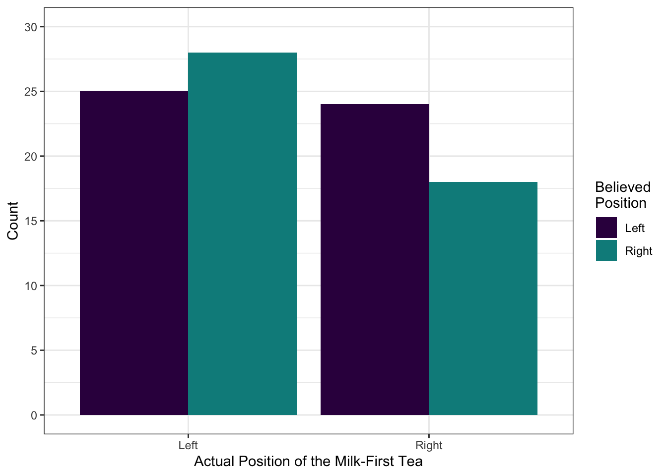
Let’s build a beautiful plot to represent the count data we have. We’ll start with a basic plot and build it up from there to create a publication-worthy graph. Along the way, we’ll learn a few new options in ggplot2. In the end, it will look like this:
Task 3
Create a bar chart.
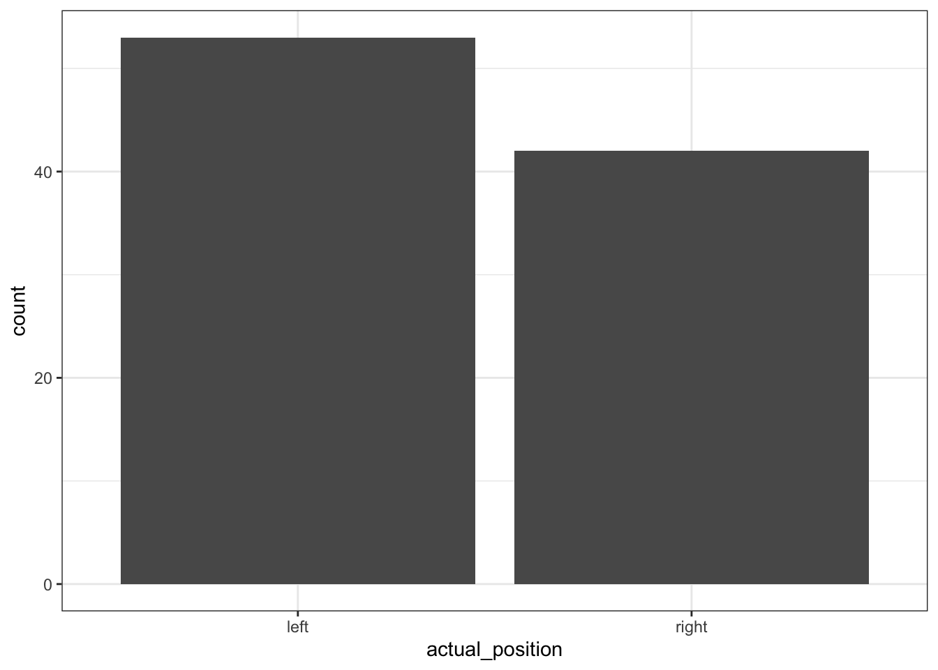
Start by creating a basic bar chart of the actual_position variable like the one below, and adding a theme to spruce it up.
- Create a base layer of a
ggplot, withactual_positionon the x axis. - Add
+ geom_bar()to the base layer. - Add a theme
Hint
The base layer takes the general form of:
some_dataset |> ggplot(aes(x = some_variable)) +
  ... some other code
Note that we’re not adding the y variable this time.
Solution
# create a basic bar chart
chi_tea |>
  ggplot(aes(x = actual_position)) +
  geom_bar() + # draw a bar plot
theme_bw()- In the
aes()function, add afill = believe_positionto split the x axis by this variable:
Hint
You need to add this to the base layer that you created above, inside the aes function. Remember to add a comma between arguments.
Solution
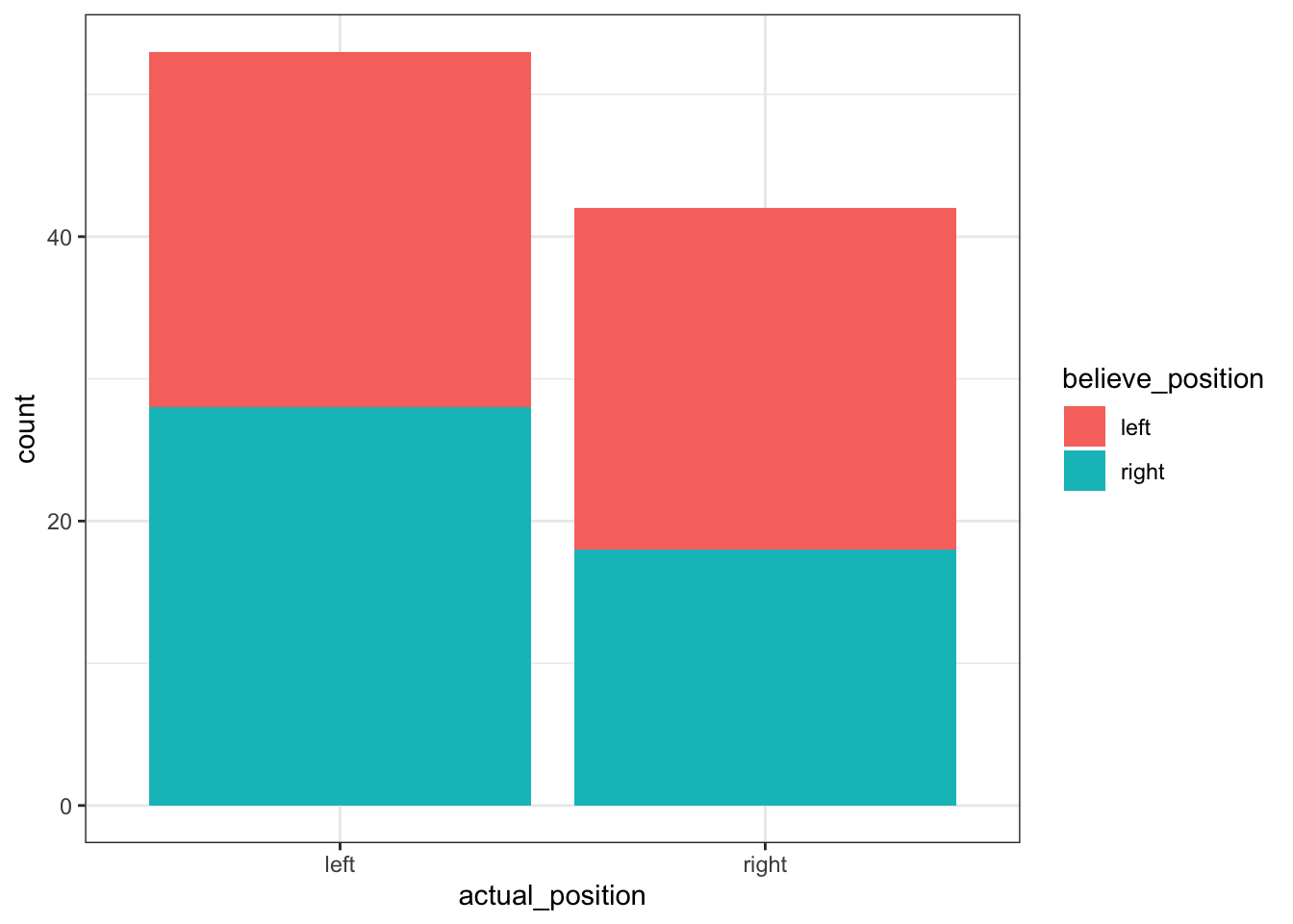
# create a basic bar chart
chi_tea |>
  ggplot(aes(x = actual_position, fill = believe_position)) +
  geom_bar() + # draw a bar plot
  theme_bw()
Hm…that doesn’t look quite right. Here, the fill argument has filled the bars with different colours. This doesn’t make comparison very easy, so instead I want to split the two bars into four, based on their value of the second variable, believe_position. In other words, I want geom_bar to draw the bars in different positions.
- Add
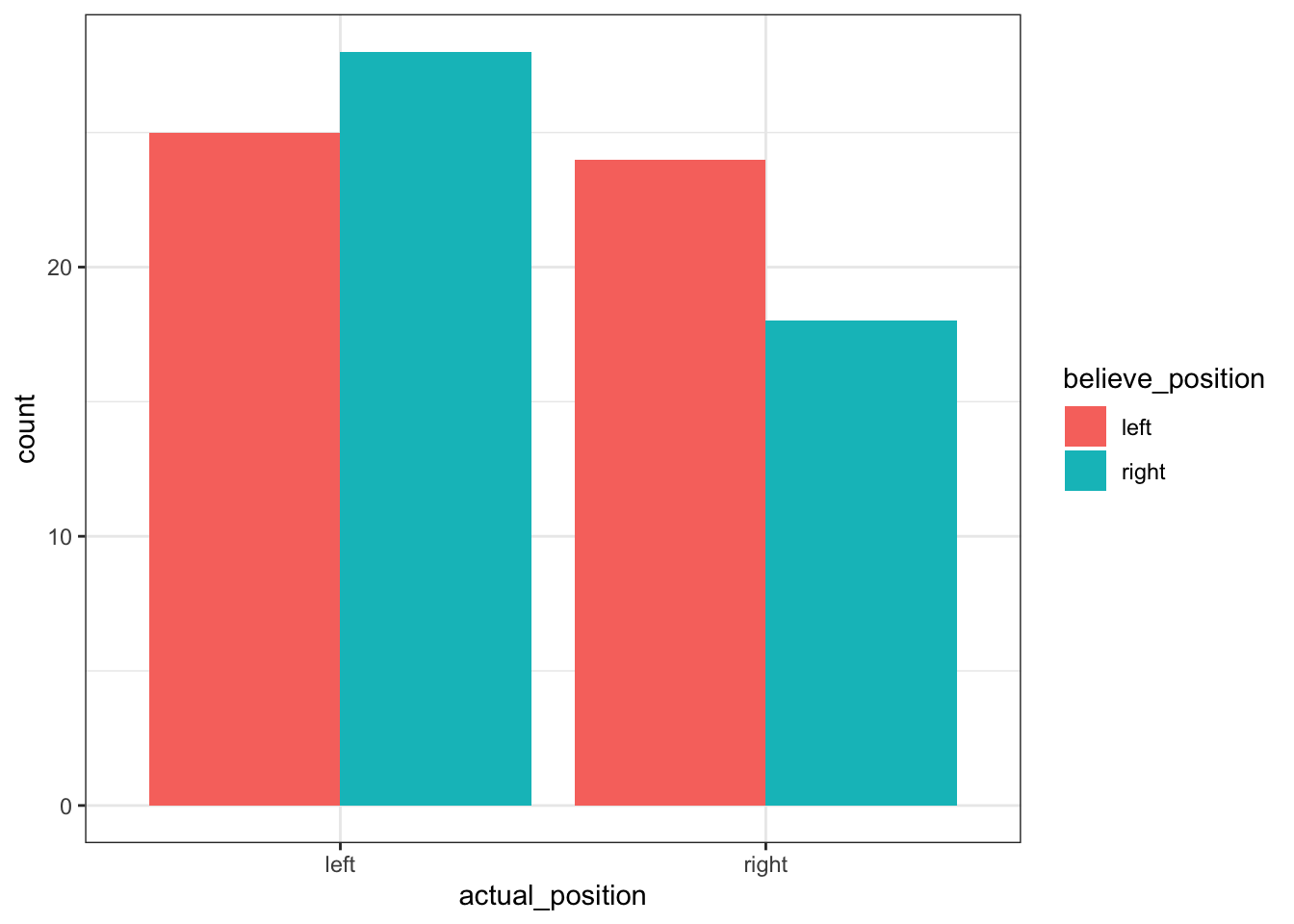
position = "dodge"to thegeom_barfunction.
Hint
You’re keeping the rest of the plot as is, but you’re adding an argument in the geom_bar() function, which was previously empty.
Solution
# create a basic bar chart
chi_tea |>
  ggplot(aes(x = actual_position, fill = believe_position)) +
  geom_bar(position = "dodge") + # draw a bar plot
  theme_bw()
Hey, that’s looking better already! That’s basically the information that we want, and this would be enough if we were just using this graph to visualise the data for our own purposes. However, we’re practicing making our plots ✨snazzy✨, so let’s keep working on making it look good.
- Change the labels using the functions
scale_x_discrete(),scale_y_continuous(),scale_fill_discrete().
scale_x_discrete()to change the name and labels on the x-axisscale_y_continuous()to change the name, limits, and breaks on the y-axisscale_fill_discrete()to change the name and labels on the legend
- Change the colours: Add a
type = c(...argument toscale_fill_discrete()to change the colours. Remember you will need to give two colours, one for “left” and one for “right”.
Hint
This is quite a lot! The next hint will show you the full structure of what the code is supposed to look like. If you want to keep it hardcore, there are some smaller hints below. Also check out the section: “More on scale_...() functions”.
The arguments in each of the scaling functions are exactly as they are listed in the instructions
Any names and labels will need to be in double quotes. If you’re adding more than one name or colour, remember to wrap them in the
c()function,Both
limitsandbreaksare numeric arguments.
Next
The full code should be structured as follows:
some_code |>
  ggplot(aes(x = x_variable, fill = fill_variable)) + # you've done these already
  geom_bar(position = "dodge") +
  scale_x_discrete(name = "Label for the X axis", # something like "actual position"
                   labels = c("label_1", "label_2")) + # what are the two possible positions?
  scale_y_continuous(name = "Count", # label for y.
                     limits = c(min_val, max_val),  # what is the minimum and the maximum you want to display? change these to numbers
                     breaks = seq(min_val, max_val, by = by_val)) + # breaks are the ticks on the plot. Usually min_val is 0, max_val is the maximum value displayed and by_val tells R how often the ticks should appear. ("E.g, show a tick at every 5th value")
  scale_fill_discrete(name = "Label for fill", # label for the second variable
                      labels = c("label_1", "label_2"),# labels for the positions
                      type = c("colour_one", "colour_two")) + # pick two colours here
  theme_SOMETHING() # change SOMETHING here to a valid theme
Solution
# tweak axis scales and labels
chi_tea |>
  ggplot(aes(x = actual_position, fill = believe_position)) +
  geom_bar(position = "dodge") +
  scale_x_discrete(name = "Actual Position of the Milk-First Tea",
                   labels = c("Left", "Right")) +
  scale_y_continuous(name = "Count",
                     limits = c(0, 30),
                     breaks = seq(0, 35, by = 5)) +
  scale_fill_discrete(name = "Believed Position",
                      labels = c("Left", "Right"),
                      type = c("#36024d", "darkcyan")) +
  theme_bw()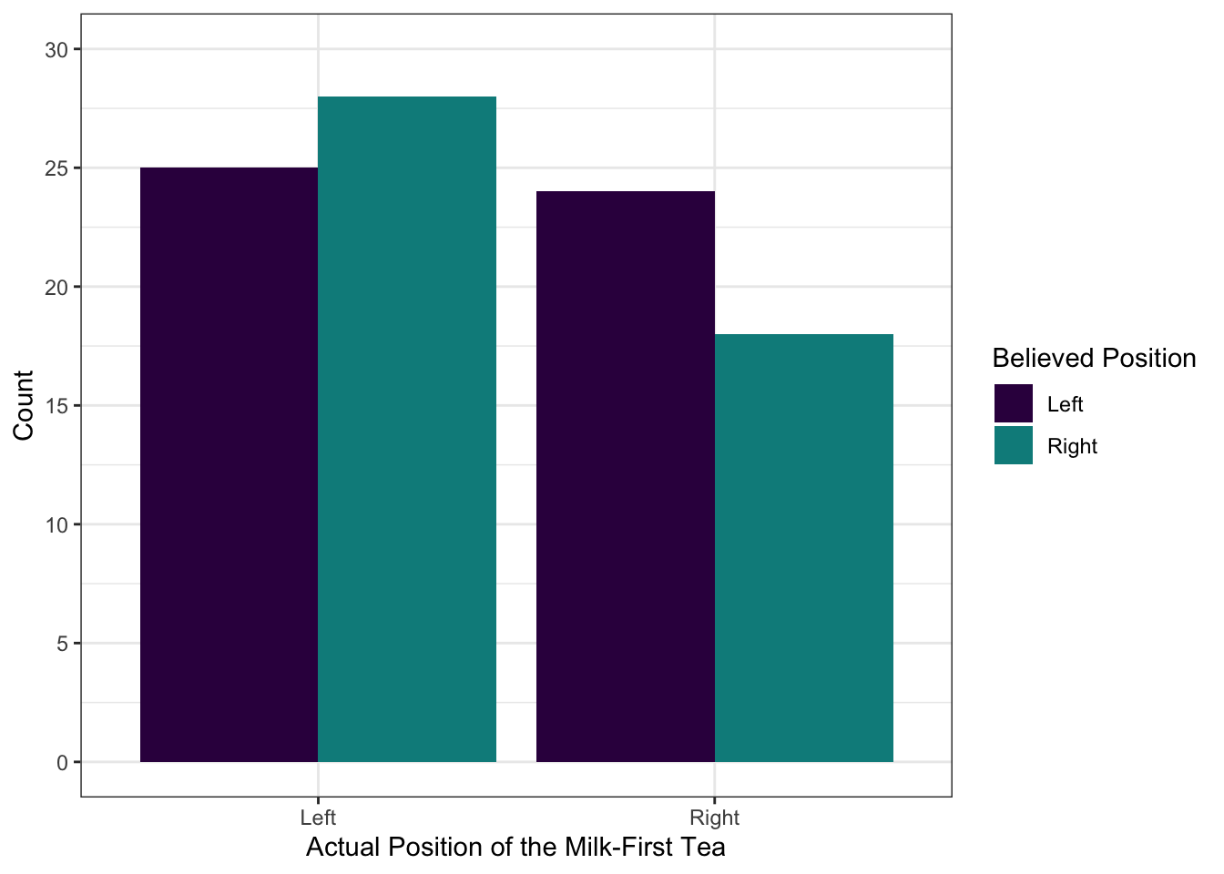
Now that’s looking good!
More on
scale_...() functions
We’ve just seen a couple of examples of functions with different names, that all follow a specific pattern. These scale_...() functions adjust the settings of the axes, as we just saw, but you have to choose the right one based on two elements:
Which axis you want to change. This is the middle element, between the underscores. Here we had
_x_for the x-axis,_y_for the y-axis, and_fill_for the grouping variable. Notice that these are the same names as the arguments in theaes()function! For example, since we putbelieve_positionin thefill =arguments inaes(), we have to use thescale_fill_...()function to change its settings.What kind of data you have. This is the last element, before the round brackets. Here we saw
_discretefor categorical data, and_continuousfor continuous data.
In order to choose the correct scale_...() variable, you have to know both of these things! R will complain if you try to use a function that doesn’t match up with the data you have.
Task 4
- Interpret the results based on the plot
- Write down your thoughts in your Quarto Doc
Hint
You need to look at how tall the bars are and whether the differences in the different colour bars are similar
Solution
To interpret the plot, look at one bit of it at a time. So, let’s look at the scenario where the milk-first tea was actually on the participant’s left. In this case, people actually thought it was on the right slightly more often than they thought it was on the left. If we look at the other half of the plot, when the milk-first tea was on the right, people tended to believe it was the one on the left!
Overall, people were incorrect more often than they were correct - but not by much, as we can tell because the bars are of fairly similar heights.
Chai-Square3 Analysis
So, we’ve made our predictions, and we’ve had a look at the data. Now we’re ready to conduct our \(\chi^2\) test.
Task 5
Perform the \(\chi^2\) analysis
- Use the
chisq.test()function to perform a \(\chi^2\) test of association on thechi_teadata. The way to specify the variables is a little different than we’re used to - check the help documentation if you get stuck! - Save your test output to a new object,
chi_tea_test, to refer to it later. - Print the results
Hint
All you need to put into the chisq.test() function are the two variables we are using. You should use subsetting with $ here; this function doesn’t play well with pipes!
Solution
# run a chi-square test
chi_tea_test <- chisq.test(chi_tea$actual_position, chi_tea$believe_position)

# Print the results
chi_tea_test
    Pearson's Chi-squared test with Yates' continuity correction

data:  chi_tea$actual_position and chi_tea$believe_position
X-squared = 0.57655, df = 1, p-value = 0.4477
Pretty painless, eh?
Reporting \(\chi^2\) Analysis
Now that we’ve got our test result, let’s report it in APA style. This takes the general form:
General Format for Reporting Statistical Results
(name_of_estimate(degrees_of_freedom) = value_of_estimate, p = exact_p, 95% CI [lower_bound, upper_bound])
Task 6
Report the results of the analysis
- Use the general format above and the values to type out the result of the \(\chi^2\) test.
- We should also describe in words what this result means. We essentially include the statistical result as a citation to give evidence for our claim. Have a go writing out a report of this statistical analysis.
Solution
We start with the general form:
name_of_test_statistic(degrees_of_freedom) = value_of_test_statistic, p = exact_p
Now we need each of these values from the output:
name_of_test_statistic: \(\chi^2\)
degrees_of_freedom: 1
value_of_test_statistic: 0.58
p: .448
So, our reporting should look like: \(\chi^2\) (1) = 0.58, p = .448
Note: write \(\chi^2\) by typing $\chi^2$ in your Markdown!
That’s good progress! However, as mentioned in the lecture, just this test isn’t enough to fully understand the results of our study. This only tells us whether the two variables were associated, not the direction of the association. For a complete report, we should also include the observed frequencies.
Caution
You should never have any raw (unformatted) code or output in a report! Always report results in the text, in a figure, or in a formatted table.
Observed and Expected Frequencies
To finish off our reporting, it’s good practice to report the actual numbers or frequencies that went into the chi-squared test. Luckily, we can get this very easily out of the chi_tea_test object we created earlier.
Task 7
Obtain and report observed and expected frequencies
- Use
str()to look at the structure of thechi_tea_testobject.
- Print out the table of observed frequencies by pulling out
$ observedfrom thechi_tea_testobject.
- Check the
expectedfrequencies for your test. Is there a problem? - Put all of this together into one report of your findings that includes information about frequencies.
Solution
# look at the structure of chi_tea_test
str(chi_tea_test)
List of 9
$ statistic: Named num 0.577
..- attr(*, "names")= chr "X-squared"
$ parameter: Named int 1
..- attr(*, "names")= chr "df"
$ p.value : num 0.448
$ method : chr "Pearson's Chi-squared test with Yates' continuity correction"
$ data.name: chr "chi_tea$actual_position and chi_tea$believe_position"
$ observed : 'table' int [1:2, 1:2] 25 24 28 18
..- attr(*, "dimnames")=List of 2
.. ..$ chi_tea$actual_position : chr [1:2] "left" "right"
.. ..$ chi_tea$believe_position: chr [1:2] "left" "right"
$ expected : num [1:2, 1:2] 27.3 21.7 25.7 20.3
..- attr(*, "dimnames")=List of 2
.. ..$ chi_tea$actual_position : chr [1:2] "left" "right"
.. ..$ chi_tea$believe_position: chr [1:2] "left" "right"
$ residuals: 'table' num [1:2, 1:2] -0.447 0.502 0.461 -0.518
..- attr(*, "dimnames")=List of 2
.. ..$ chi_tea$actual_position : chr [1:2] "left" "right"
.. ..$ chi_tea$believe_position: chr [1:2] "left" "right"
$ stdres : 'table' num [1:2, 1:2] -0.966 0.966 0.966 -0.966
..- attr(*, "dimnames")=List of 2
.. ..$ chi_tea$actual_position : chr [1:2] "left" "right"
.. ..$ chi_tea$believe_position: chr [1:2] "left" "right"
- attr(*, "class")= chr "htest"# print observed frequencies
chi_tea_test$observed chi_tea$believe_position
chi_tea$actual_position left right
left 25 28
right 24 18# print expected frequencies
chi_tea_test$expected chi_tea$believe_position
chi_tea$actual_position left right
left 27.33684 25.66316
right 21.66316 20.33684You might notice that the observed values are the same counts that appeared in our graph up above. Even though this information is presented visually there, it’s still a good idea to include these numbers in your report.
More about
htest objects
The object we’ve created to store the results of our test, which we’ve called chi_tea_test, is in essence just a list of values that were calculated by the test. This particular list has a special class, htest, for hypothesis tests. If you look back on previous work, you’ll see that our objects containing the results from t.test() and cor.test() were also htest objects.
The benefit of being familiar with htest objects is that they all work in a similar way. They are all lists of information - more information than it appears when you just call the object and print out the test results!
In this case, our output from chisq.test() has some elements that are incredibly useful but not printed by default: $observed and $expected, which contain the observed and expected frequencies respectively. So, it’s a good idea to have a look inside these objects when you are reporting - it will often make your life a bit easier!
Recap
Well done conducting your \(\chi^2\) analysis. I highly recommend reading all of the T3 Team’s findings - they asked a lot of interesting questions and have done a great job presenting their results.
In sum, we’ve covered:
How to create bar graphs of count data
How to run the \(\chi^2\) analysis, read the output, and store it in an object
How to report and interpret the statistical results of these tests in real-world terms
Remember, if you get stuck or you have questions, post them on Discord, or bring them to practicals or to drop-ins.
Good job!
That’s all for today. See you soon!
ChallengR
ChallengR Time!
This task is a ChallengR, which are always optional, and will never be assessed - they’re only there to inspire you to try new things! If you solve this task successfully, you can earn a bonus 2500 Kahoot Points. You can use those points to earn bragging rights and, more importantly, shiny stickers. (See the Games and Awards page on Canvas.)
There are no solutions in this document for this ChallengR task. If you get stuck, ask us for help in your practicals or at the Help Desk, and we’ll be happy to point you in the right direction.
Task 8
Research question
Is there a statistically significant association between the types of game played (shooter vs RPG) and different age categories (under 35, 35-45, over 45)?
Your task is to answer the research question above. In doing so, complete the following steps and then answer the questions in the Week 7 ChallengR Canvas quiz.
- Read in the data using the code below.
- Check whether you need to make any changes to the dataset before running the test. If so, carry out these changes.
- Create a summary table that shows you the counts of individuals within the two game types and the three age categories.
- Run a statistical test to answer the research question.
- Optional: Create an appropriate data visualisation to help you interpret the results.
# load data:
games_tib <- readr::read_csv("data/video_games_data.csv")
Once you’re happy with your code, complete the quiz on Canvas to those well-deserved Kahoot points: Week 7 ChallengR quiz on Canvas. Good luck, and well done again!
Footnotes
In L’s words, just now watching it again: “How did she get every single bit of it wrong?” And L doesn’t even drink tea!↩︎