library(tidyverse)Tutorial 04: Summarising data
Introduction
In previous tutorials, we’ve learned about several useful functions from dplyr used for selecting variables, searching for cases that meet specific conditions, and creating new variables. At this point, we know how to search through data and work with datasets, but how do we start making sense of it all? This is where we need to start thinking about summarising data, which is what this tutorial covers. To make things more fun, we’ll pair some new dplyr functions with the pipe |>, which we’ve learned about in the previous tutorial. We’ll end with some easy functions for making these summary tables pretty, and some optional extras about plotting and interpreting CIs.
Data
In late 2023, some reputable newspapersTM started reporting a new strategy that sailors had implemented for deterring orcas1 that frequently attacked boats - heavy metal. Some sailors noticed that orca attacks tended to last shorter than usual if they were blasting heavy metal music. Others however, had a vastly different experience.
The Analysing Data team was hired by the South Pole Sailors’ Society to sail through the waters of Gibraltar, collect some high quality data, and settle the debate once and for all. We collected information about over 150 attacks. During each attack, we either played metal music from various bands, or the soundtrack from the movie Shrek. Now we can look at the general trends in the data and produce some summaries.
Task 1
Load packages and explore the dataset.
- Load the
tidyverse. - The dataset file can be found on the path
data/orca_data.csv. Usereadr::read_csv()to read the data in. - Store the dataset in an object called
orca_tibso we can use it later. - Explore the dataset to become familiar with the variables.
Hint
You’ll need to use the library() function to load packages. This function needs to be called somewhere at the beginning of the document.
Next
You can read datasets with readr::read_csv(). Have a look at previous weeks’ code for examples!
Solution
Load packages:
Load the dataset:
orca_tib <- readr::read_csv("data/orca_data.csv")Exploring the data - there are several things you could try here. Some options include:
orca_tib- Calling the name of the dataset will print the whole dataset, 10 rows at the timeView(orca_tib)- will open the data in the viewer. It’s better to only use this option in the console and not in the document itself. Weird things happen if you try to render a document that contains theView()function.
| attack_id | date_of_attack | month | attack_duration | music_genre | band |
|---|---|---|---|---|---|
| 12 | 2020-10-03 | 10 | 58 | Genre Mix | NA |
| 18 | 2020-10-14 | 10 | 51 | Heavy Metal | NA |
| 19 | 2020-10-16 | 10 | 40 | Heavy Metal | Opeth |
| 21 | 2020-10-21 | 10 | 44 | Heavy Metal | NA |
| 23 | 2020-10-23 | 10 | 53 | Genre Mix | NA |
| 24 | 2020-10-24 | 10 | 52 | Heavy Metal | Saor |
| 26 | 2020-10-27 | 10 | 55 | Genre Mix | NA |
| 29 | 2020-11-02 | 11 | 52 | Genre Mix | NA |
| 33 | 2020-11-11 | 11 | 45 | Genre Mix | NA |
| 34 | 2020-11-17 | 11 | 43 | Genre Mix | NA |
| 36 | 2020-11-24 | 11 | 44 | Genre Mix | NA |
| 41 | 2020-12-17 | 12 | 44 | Heavy Metal | Powerwolf |
| 42 | 2020-12-18 | 12 | 54 | Genre Mix | NA |
| 46 | 2020-12-29 | 12 | 50 | Genre Mix | NA |
| 48 | 2021-01-02 | 1 | 23 | Heavy Metal | Opeth |
| 55 | 2021-01-18 | 1 | 43 | Heavy Metal | Powerwolf |
| 57 | 2021-01-25 | 1 | 44 | Heavy Metal | Saor |
| 59 | 2021-01-29 | 1 | 43 | Genre Mix | NA |
| 60 | 2021-02-08 | 2 | 47 | Genre Mix | NA |
| 62 | 2021-02-10 | 2 | 19 | Heavy Metal | Opeth |
| 65 | 2021-02-27 | 2 | 37 | Genre Mix | NA |
| 76 | 2021-03-30 | 3 | 50 | Genre Mix | NA |
| 80 | 2021-04-18 | 4 | 32 | Heavy Metal | Powerwolf |
| 86 | 2021-05-02 | 5 | 44 | Genre Mix | NA |
| 90 | 2021-05-15 | 5 | 30 | Heavy Metal | Opeth |
| 92 | 2021-05-21 | 5 | 47 | Genre Mix | NA |
| 100 | 2021-06-02 | 6 | 64 | Genre Mix | NA |
| 101 | 2021-06-04 | 6 | 31 | Heavy Metal | Iron Maiden |
| 105 | 2021-06-11 | 6 | 61 | Genre Mix | NA |
| 106 | 2021-06-12 | 6 | 37 | Genre Mix | NA |
| 107 | 2021-06-13 | 6 | 51 | Genre Mix | NA |
| 108 | 2021-06-14 | 6 | 30 | Heavy Metal | Iron Maiden |
| 110 | 2021-06-18 | 6 | 45 | Heavy Metal | Powerwolf |
| 111 | 2021-06-19 | 6 | 25 | Genre Mix | NA |
| 118 | 2021-07-01 | 7 | 27 | Heavy Metal | Iron Maiden |
| 122 | 2021-07-09 | 7 | 42 | Heavy Metal | Opeth |
| 125 | 2021-07-15 | 7 | 43 | Genre Mix | NA |
| 131 | 2021-07-30 | 7 | 41 | Heavy Metal | Saor |
| 133 | 2021-08-05 | 8 | 42 | Genre Mix | NA |
| 142 | 2021-08-28 | 8 | 57 | Heavy Metal | Saor |
| 143 | 2021-08-30 | 8 | 59 | Genre Mix | NA |
| 146 | 2021-09-13 | 9 | 29 | Heavy Metal | Powerwolf |
| 147 | 2021-09-14 | 9 | 67 | Genre Mix | NA |
| 158 | 2021-10-10 | 10 | 37 | Heavy Metal | Saor |
| 161 | 2021-10-17 | 10 | 53 | Heavy Metal | Opeth |
| 166 | 2021-11-02 | 11 | 64 | Genre Mix | NA |
| 167 | 2021-11-03 | 11 | 38 | Heavy Metal | Opeth |
| 169 | 2021-11-09 | 11 | 71 | Heavy Metal | Saor |
| 171 | 2021-11-15 | 11 | 50 | Genre Mix | NA |
| 174 | 2021-11-26 | 11 | 41 | Heavy Metal | NA |
| 177 | 2021-12-01 | 12 | 60 | Genre Mix | NA |
| 181 | 2021-12-13 | 12 | 59 | Genre Mix | NA |
| 183 | 2021-12-19 | 12 | 42 | Heavy Metal | Saor |
| 186 | 2021-12-31 | 12 | 44 | Genre Mix | NA |
| 189 | 2022-01-09 | 1 | 26 | Heavy Metal | Iron Maiden |
| 191 | 2022-01-11 | 1 | 66 | Genre Mix | NA |
| 194 | 2022-01-15 | 1 | 25 | Heavy Metal | Saor |
| 196 | 2022-01-19 | 1 | 51 | Genre Mix | NA |
| 198 | 2022-01-26 | 1 | 23 | Heavy Metal | Iron Maiden |
| 202 | 2022-02-05 | 2 | 44 | Heavy Metal | NA |
| 207 | 2022-02-20 | 2 | 36 | Genre Mix | NA |
| 210 | 2022-03-08 | 3 | 41 | Genre Mix | NA |
| 214 | 2022-03-17 | 3 | 50 | Genre Mix | NA |
| 217 | 2022-03-20 | 3 | 47 | Genre Mix | NA |
| 218 | 2022-03-25 | 3 | 36 | Heavy Metal | Saor |
| 220 | 2022-03-27 | 3 | 35 | Genre Mix | NA |
| 221 | 2022-03-28 | 3 | 51 | Heavy Metal | NA |
| 225 | 2022-04-02 | 4 | 27 | Heavy Metal | Iron Maiden |
| 235 | 2022-04-25 | 4 | 41 | Genre Mix | NA |
| 236 | 2022-04-26 | 4 | 37 | Heavy Metal | NA |
| 237 | 2022-05-03 | 5 | 50 | Heavy Metal | Saor |
| 243 | 2022-05-22 | 5 | 58 | Heavy Metal | NA |
| 245 | 2022-05-26 | 5 | 34 | Heavy Metal | Iron Maiden |
| 247 | 2022-05-31 | 5 | 42 | Genre Mix | NA |
| 248 | 2022-06-05 | 6 | 39 | Heavy Metal | Saor |
| 255 | 2022-07-07 | 7 | 36 | Heavy Metal | Opeth |
| 256 | 2022-07-09 | 7 | 45 | Genre Mix | NA |
| 257 | 2022-07-11 | 7 | 40 | Heavy Metal | Saor |
| 262 | 2022-07-19 | 7 | 49 | Heavy Metal | Iron Maiden |
| 268 | 2022-08-02 | 8 | 52 | Heavy Metal | Opeth |
| 270 | 2022-08-05 | 8 | 52 | Heavy Metal | NA |
| 271 | 2022-08-06 | 8 | 27 | Heavy Metal | Opeth |
| 273 | 2022-08-09 | 8 | 30 | Heavy Metal | Iron Maiden |
| 275 | 2022-08-11 | 8 | 48 | Genre Mix | NA |
| 280 | 2022-08-21 | 8 | 28 | Heavy Metal | Powerwolf |
| 282 | 2022-08-24 | 8 | 55 | Heavy Metal | NA |
| 285 | 2022-09-02 | 9 | 61 | Heavy Metal | Iron Maiden |
| 286 | 2022-09-10 | 9 | 38 | Genre Mix | NA |
| 288 | 2022-09-13 | 9 | 55 | Heavy Metal | NA |
| 290 | 2022-09-18 | 9 | 40 | Heavy Metal | Powerwolf |
| 291 | 2022-09-19 | 9 | 41 | Genre Mix | NA |
| 296 | 2022-10-04 | 10 | 37 | Heavy Metal | Iron Maiden |
| 300 | 2022-10-18 | 10 | 42 | Heavy Metal | NA |
| 306 | 2022-10-31 | 10 | 68 | Genre Mix | NA |
| 308 | 2022-11-03 | 11 | 60 | Heavy Metal | NA |
| 309 | 2022-11-08 | 11 | 46 | Heavy Metal | NA |
| 311 | 2022-11-11 | 11 | 57 | Heavy Metal | NA |
| 313 | 2022-11-14 | 11 | 72 | Genre Mix | NA |
| 314 | 2022-11-18 | 11 | 68 | Genre Mix | NA |
| 315 | 2022-11-19 | 11 | 44 | Heavy Metal | Iron Maiden |
| 316 | 2022-11-22 | 11 | 47 | Genre Mix | NA |
| 319 | 2022-11-26 | 11 | 39 | Heavy Metal | Iron Maiden |
| 320 | 2022-11-27 | 11 | 33 | Heavy Metal | Iron Maiden |
| 321 | 2022-11-28 | 11 | 32 | Heavy Metal | Iron Maiden |
| 323 | 2022-12-03 | 12 | 54 | Genre Mix | NA |
| 327 | 2022-12-07 | 12 | 41 | Heavy Metal | Opeth |
| 328 | 2022-12-11 | 12 | 57 | Heavy Metal | NA |
| 330 | 2022-12-15 | 12 | 36 | Heavy Metal | Iron Maiden |
| 337 | 2022-12-26 | 12 | 53 | Heavy Metal | Powerwolf |
| 341 | 2023-01-12 | 1 | 45 | Heavy Metal | Saor |
| 348 | 2023-01-24 | 1 | 31 | Genre Mix | NA |
| 349 | 2023-01-26 | 1 | 31 | Heavy Metal | Iron Maiden |
| 350 | 2023-01-27 | 1 | 42 | Genre Mix | NA |
| 351 | 2023-01-29 | 1 | 27 | Heavy Metal | Iron Maiden |
| 352 | 2023-01-30 | 1 | 39 | Heavy Metal | Saor |
| 357 | 2023-02-12 | 2 | 46 | Heavy Metal | NA |
| 358 | 2023-02-13 | 2 | 38 | Heavy Metal | Saor |
| 359 | 2023-02-15 | 2 | 76 | Genre Mix | NA |
| 360 | 2023-02-16 | 2 | 38 | Heavy Metal | Opeth |
| 363 | 2023-02-19 | 2 | 22 | Heavy Metal | NA |
| 370 | 2023-03-05 | 3 | 63 | Genre Mix | NA |
| 371 | 2023-03-08 | 3 | 27 | Heavy Metal | Powerwolf |
| 373 | 2023-03-10 | 3 | 50 | Genre Mix | NA |
| 380 | 2023-03-19 | 3 | 38 | Genre Mix | NA |
| 384 | 2023-03-31 | 3 | 41 | Genre Mix | NA |
| 385 | 2023-04-02 | 4 | 44 | Heavy Metal | Iron Maiden |
| 398 | 2023-05-01 | 5 | 62 | Genre Mix | NA |
| 404 | 2023-05-21 | 5 | 63 | Genre Mix | NA |
| 407 | 2023-05-25 | 5 | 53 | Genre Mix | NA |
| 409 | 2023-05-30 | 5 | 39 | Genre Mix | NA |
| 410 | 2023-06-11 | 6 | 44 | Heavy Metal | NA |
| 413 | 2023-06-19 | 6 | 51 | Heavy Metal | Saor |
| 414 | 2023-06-20 | 6 | 54 | Genre Mix | NA |
| 418 | 2023-06-24 | 6 | 51 | Genre Mix | NA |
| 424 | 2023-07-10 | 7 | 36 | Heavy Metal | Powerwolf |
| 425 | 2023-07-12 | 7 | 16 | Heavy Metal | Iron Maiden |
| 426 | 2023-07-18 | 7 | 49 | Heavy Metal | NA |
| 427 | 2023-07-25 | 7 | 43 | Genre Mix | NA |
| 428 | 2023-07-26 | 7 | 66 | Genre Mix | NA |
| 429 | 2023-07-27 | 7 | 12 | Heavy Metal | Iron Maiden |
| 433 | 2023-08-01 | 8 | 55 | Genre Mix | NA |
| 434 | 2023-08-02 | 8 | 47 | Genre Mix | NA |
| 435 | 2023-08-11 | 8 | 52 | Genre Mix | NA |
| 440 | 2023-08-28 | 8 | 48 | Heavy Metal | Saor |
| 443 | 2023-09-13 | 9 | 56 | Genre Mix | NA |
| 444 | 2023-09-14 | 9 | 52 | Heavy Metal | Saor |
| 446 | 2023-09-23 | 9 | 40 | Heavy Metal | Saor |
| 448 | 2023-10-09 | 10 | 43 | Heavy Metal | Opeth |
| 449 | 2023-10-11 | 10 | 41 | Heavy Metal | Saor |
| 452 | 2023-10-22 | 10 | 40 | Genre Mix | NA |
| 454 | 2023-10-24 | 10 | 44 | Heavy Metal | Opeth |
| 458 | 2023-10-31 | 10 | 28 | Heavy Metal | Opeth |
| 460 | 2023-11-02 | 11 | 45 | Genre Mix | NA |
| 462 | 2023-11-10 | 11 | 46 | Genre Mix | NA |
| 463 | 2023-11-11 | 11 | 60 | Genre Mix | NA |
| 464 | 2023-11-12 | 11 | NA | Heavy Metal | Powerwolf |
| 465 | 2023-11-14 | 11 | 50 | Genre Mix | NA |
| 466 | 2023-11-17 | 11 | 34 | Heavy Metal | Iron Maiden |
| 467 | 2023-11-18 | 11 | 58 | Genre Mix | NA |
| 470 | 2023-11-21 | 11 | 59 | Genre Mix | NA |
| 477 | 2023-12-09 | 12 | 61 | Genre Mix | NA |
| 478 | 2023-12-10 | 12 | 40 | Heavy Metal | Opeth |
| 484 | 2023-12-24 | 12 | 45 | Heavy Metal | Powerwolf |
| 485 | 2023-12-26 | 12 | 39 | Genre Mix | NA |
Codebook
attack_id- ID number of the orca attackdate_of_attack- date when the attack happenedmonth- month when the attack was recorded. Numeric (1 - January, 12 - December)attack_duration- duration of the attack in minutesmusic_genre- did the crew play heavy metal or Shrek soundtracks during the attacks?band- name of the band
Research Question
Before we jump into the code, let’s first think for a moment about what we’re going to do and why.
We have our dataset, which was described by the Codebook above. From next week, we’ll start doing statistical testing on datasets like, this, but summarising your data, using “descriptives”, is absolutely essential before we start. These descriptives, which are the main focus of today’s tutorial, describe your data, often using measures of central tendency and other ways to quantify the data you have. The summary values you include in “descriptives” will vary, depending on your dataset and the things you want to know. So, before we do anything else, we need to figure out what we want know. Have a go at the quiz below, and refer to the Introduction if you don’t remember some details.
This setup - comparing some score, behaviour, latency etc. between two independent conditions - is an extremely common and useful study format in Psychology and in science generally. So much so, we’ll continue to work on this same design next week! For now, we still have some thinking to do.
Task 2
Referring to the Introduction and what you have learned about the study design thus far, what descriptive information would be useful in order to investigate the research question? Make a list in your notebook document and explain why you included each element.
Hint
Hi again! It’s tempting to skip tasks like this, but we strongly recommend you don’t. The practice will come in handy in the future - that is a threat promise 👀
If you need a refresher on descriptive statistics, look back on Lectures 6 and 7 of Psychology as a Science for some good options. There was also a new descriptive measure introduced in this week’s lecture that you may consider including.
Solution
To start, we already identified the two key variables we’re interested in from the quiz above. As a reminder, we want to know about the duration of orca attacks when we are playing metal music, vs when we are playing the Shrek soundtrack. Here, the duration of attacks is the key thing we really want to know about. So, how can we summarise, or describe, this variable?
If you’re feeling a bit stumped, the first thing we can do is think about the measures of central tendency from Week 5 of PAAS. In that lecture, there were three key techniques covered: mean, median, and mode. This lecture mentions that the mean is often preferred, because it takes all the observations into consideration and essentially captures the typical value in a sample. (You may have noticed that the mean comes up a lot, and we will see more of it in the future!) That sounds great, so one of the main things we’ll want to include is the mean of attack duration.
In the PAAS lecture, we also saw however that the mean is sensitive to outliers. This means that if there are extreme or unusual values in the dataset that are quite different from all the others, the mean that we calculate for that sample might be very different than it would be if just those few extreme values weren’t there. In other words, if we just looked at the mean, it could be misleading without other information. So, what other information might be useful?
In addition to the mean, it’s a good idea to get some measures of how much the scores are spread around the mean. Some very simple examples of this are the range, or minimum and maximum values, which are simply the highest and lowest values in the sample. Since these are the most extreme values, if these values are very small (or very big), they might tip us off that something’s going on in the data we need to look into.
A more sophisticated measure is the standard deviation, which is almost always reported alongside the mean. The standard deviation tells us how much the values in the sample differ from the mean of those values, on average. It’s a useful way to capture whether the values tend to be quite similar to the mean, so the mean represents the sample well (in which case the SD will be small); or if the values tend to be quite different from the mean, so the mean doesn’t represent the sample well (in which case the SD will be large).
It’s often a good idea to obtain the median, another measure of central tendency. The mean will be our key descriptive measure, but ideally if our values are normally distributed, the mean and the median should be quite similar to each other. If they aren’t, that might suggest that the data are skewed - that is, there tend to be more or less of certain values than we expected.
In this week’s lecture we also introduced confidence intervals (CIs), which we will explore in more depth in just a bit.
Finally, we’re interested in all of these measures both overall, and for the two music genre groups separately, so we can compare them.
To practice, try making a short list of each of the descriptive measures we’ve talked about here to refer to later on. It would be a good idea to summarise why each one should be included and what information it contributes…you know, in case you need it someday…👀
Now that we have an idea of what we are doing and why, let’s get going in R!
Overall Summaries with summarise()
Before we dive into comparing the two groups, it’s good practice to create some general summaries for our whole sample. Different descriptive statistics are useful in different situations. For our purposes, we want to create a table that contains the values we listed above:
Number of cases
Minimum and maximum values for
attack_durationMean, median, and standard deviation for
attack_durationConfidence intervals for
attack_duration
Basic Form
To create summary tables, we can use the summarise() function from the dplyr package. The summarise() function works very similarly to mutate(). We start by telling the function which dataset we want to use with the .data = argument, and then we give instructions for what kind of summary value we want to create and how we want to call a column that contains this value.
A code creating a basic summary table looks like this:
dplyr::summarise(
  .data = our_dataset,
  summary_column_name = some_function
)
In the last tutorial, we’ve also introduced the pipe operator, which looks like this: |>. The pipe operator is very handy once our code starts getting bulky - it makes our code more efficient and easy to read. So let’s re-write the summary code above to use the pipe:
some_dataset |>
  dplyr::summarise(
    summary_column_name = some_function
  )
Notice that the .data argument has now disappeared. That’s because it’s the first argument - functions in R automatically pipe the object on the left hand side (in this case some_dataset) into the first unnamed argument, so we don’t need to specify it anymore.
Now let’s adapt this code to create some actual summaries.
Counting Cases
We’ll start by counting the number of cases in the dataset, which we’ll store in a new column we can call n_cases. The function we can use for this is the n() function from the {dplyr} package. dplyr::n() is a bit of a funny function, in that it doesn’t take any arguments and can only be used inside of other {dplyr} functions. We therefore don’t need to modify the function itself. In this scenario, we only need to change the dataset name and the variable name for our code to work.
Task 3
Copy the code below and then replace the dataset name and the summary column name with appropriate values. Run the code in your .qmd file to see the results.
# create a table containing the number of participants
some_dataset |>
  dplyr::summarise(
    summary_column_name = dplyr::n()
  )
Hint
some_dataset needs to be replaced with the name of the dataset we’re using.
Next
summary_column_name can be changed to pretty much anything, but n_cases will do nicely here - it’s brief and descriptive.
Solution
The final code should look like this:
orca_tib |>
  dplyr::summarise(
    n_cases= dplyr::n()
  )
# A tibble: 1 × 1
n_cases
<int>
1 164Complete the blank: In total, there were cases in the sample.
Note that we’re not saving this summary into a new object just yet. We’re going to keep adding more summary values, and then save the finished summary object at the very end, once our code has grown a little.
MoRe About:
dplyr::n() or nrow() ?
We’ve previously learned how to get the number of participants using nrow() (see Practical 02). Here we’re using dplyr::n() combined with the dplyr::summarise() function, because it is a much more flexible approach that allows us to create summary tables containing a range of different descriptive statistics, not just the number of participants.
Descriptives
Next up, we’ll calculate some descriptive values that help us understand the data we’ve collected: minimum, maximum, mean, median, and standard deviation of attack_duration, our key variable of interest. We can tackle all of these in one section, because the functions for creating these summaries work in exactly the same way.
The minimum can be obtained using the min() function. The min() function (as well as the other functions in this section) comes from base R, so we don’t need to include a package call in front of it.
The function takes a variable name as an argument, and returns the minimum value. On its own, it can be used as:
some_variable <- c(6, 4, 1, 9, 3, 7)
min(some_variable, na.rm = TRUE)
[1] 1The minimum value in some_variable is 1, so the code above returns 1. We’ve also added the argument na.rm = TRUE, which ensures that if there are any missing values in the variable, the min() function will ignore them.
MoRe About:
na.rm = TRUE
This section is skippable if you’re happy to just keep writing na.rm = TRUE in your functions without an explanation.
We can run the code below to understand why not including na.rm=TRUE might be a problem:
orca_tib |>
  dplyr::summarise(
    min_attack= min(attack_duration)
  )
# A tibble: 1 × 1
min_attack
<dbl>
1 NAThe min value in our new summary table is returned as NA - a missing value.
An NA in a summary table often means that there’s something iffy about the variable that we’re trying to summarise. In our case, this would the attack_duration. A value of NA indicates that this variable is very likely to have some missing values.
We can use the method from explained in Tutorial 2 to explore whether attack_duration has missing values. To check for a missing values in a particular variable, we can use filter() to return any cases that DO have an NA. If the tibble is empty with no rows, there were no missing values in that variable. Otherwise, there were.
orca_tib |>
  dplyr::filter(is.na(attack_duration))
# A tibble: 1 × 6
attack_id date_of_attack month attack_duration music_genre band
<dbl> <date> <dbl> <dbl> <chr> <fct>
1 464 2023-11-12 11 NA Heavy Metal PowerwolfTurns out, attack_duration does indeed have one missing value, because this table has one row. Now, we could remove this data point from the dataset using dplyr::filter(), but let’s say that for the time being, we don’t want to discard any data.
The argument na.rm = … allows us to specify how we want to deal with the missing values. By default, this is set to FALSE. So if there are any missing values in the variable, the function will not NOT ignore them and will instead return a NA. For example:
some_variable <- c(6, 4, 1, NA, 3, 7)
min(some_variable, na.rm = FALSE)
[1] NAThe code above returns NA. Because FALSE is the default value for na.rm =, we don’t need to specify it for this behaviour to occur. The function will automatically return NA by default:
min(some_variable)[1] NABut this doesn’t help us. We want the function to ignore the missing values, and tell us the smallest value that occurs in that variable disregarding NAs. We can set the value of the na.rm argument to TRUE to achieve this behaviour:
min(some_variable, na.rm = TRUE)[1] 1If we want the summary of attack_duration, we need to add the na.rm argument to the min() function in our code.
Let’s add this function to our summary table to find out the minimum value in our dataset for attack_duration.
Task 4
Adapt the code below to create a new summary column called min_attack. The column should contain the minimum value of the attack_duration variable.
# add the minimum value to the summary table
orca_tib |>
  dplyr::summarise(
    n_cases= dplyr::n(),
    new_summary_column_name = some_code_that_returns_the_minimum
  )
Hint
new_summary_column_name can be, again, any name. You can call it jessica if you’d like and the code will work fine, but that isn’t particularly informative - that is, it doesn’t quickly and succinctly tell you what the variable name contains. What would be an informative name for a column that contains the minimum value of a variable?
Next
some_code_that_returns_the_minimum is the function that we’re using, which in this case is min(). Scroll a little bit further up to see how it can be used.
Solution
The complete code looks like this:
orca_tib |>
  dplyr::summarise(
    n_cases = dplyr::n(), ## Remember the comma!
    min_attack= min(attack_duration, na.rm = TRUE)
  )
# A tibble: 1 × 2
n_cases min_attack
<int> <dbl>
1 164 12
Remember the comma!
Note how the line with n_cases = dplyr::n(), ends with a comma. If we’re adding new summary values after a line of code inside of summarise(), we need to end that line with a comma. The last line, in this case the line that creates the minimum, doesn’t need to end with a comma. dplyr functions like summarise() will (most of the time) happily pretend that the last line doesn’t have a comma even you accidentally add one. Functions from base R tend to be less forgiving and will often return an error.
Task 5
Add the remaining summary functions. Now that you know how to to use the min() function, you can use the same formula to add the other summary values of attack_duration to the table as well. Here are the functions that you’ll need to use:
max()returns a maximum value in a variablemean()returns the variable mean (average) valuemedian()returns the mediansd()returns the standard deviation
All of these functions work in the same way when it comes to missing values, so remember to add the argument na.rm = TRUE for each of them. You can call the new columns in the summary table “max_attack”, “mean_attack”, and so on.
Hint
The first part of the code stays the same - you’ll be adding new lines after min_attack = min(attack_duration, na.rm = TRUE),.
Next
For example, to add the line that calculates the maximum value, you can write:
orca_tib |>
  dplyr::summarise(
    n_cases = dplyr::n(),
    min_attack = min(attack_duration, na.rm = TRUE),
    max_attack = max(attack_duration, na.rm = TRUE)
  )
Now try adding the remaining functions listed above in a similar way (always remember to change the column name and the function!)
Solution
The complete code looks like this:
orca_tib |>
  dplyr::summarise(
    n_cases= dplyr::n(),
    min_attack= min(attack_duration, na.rm = TRUE),
    max_attack = max(attack_duration, na.rm = TRUE),
    mean_attack = mean(attack_duration, na.rm = TRUE),
    median_attack = median(attack_duration, na.rm = TRUE),
    sd_attack = sd(attack_duration, na.rm = TRUE)
)| n_cases | min_attack | max_attack | mean_attack | median_attack | sd_attack |
|---|---|---|---|---|---|
| 164 | 12 | 76 | 44.88344 | 44 | 11.78951 |
Using the beautiful output you’ve just created, answer the following questions about the data.
Confidence Intervals
The final element that we’d like to include in our descriptives are confidence intervals. Make sure you review this week’s lecture if you don’t quite remember what confidence intervals are for, or check out the box below for a quick reminder!
MoRe About: Confidence Intervals
Confidence intervals are useful, because they allow us to infer something about the population. The lower and upper limit of a 95% confidence interval tells us the plausible range of values that the true population value could be (assuming our sample is one of the 95% producing confidence intervals that actually contain the true population value).
The function that we’re going to use to get confidence intervals into the our summary is mean_cl_normal() from the ggplot2 package.
Like the other functions, mean_cl_normal() also takes the variable names, though there’s a slight twist to it. The general use of the function is:
some_dataset |>
  dplyr::summarise(
    ci_lower = ggplot2::mean_cl_normal(variable_name)$ymin,
    ci_upper = ggplot2::mean_cl_normal(variable_name)$ymax
  )
We’re creating two summary columns, called ci_lower (“confidence interval - lower”) and ci_upper (“confidence interval - upper”). The way this function differs from the other functions is that we also need to specify whether we want the upper or the lower confidence interval. We do this by adding $ymin and $ymax, respectively, at the end of the line.
MoRe About:
$ymin and $ymax
We can have a look at the below to get some sense of how the function works:
some_variable <- c(6, 4, 1, NA, 3, 7)
ggplot2::mean_cl_normal(some_variable)| y | ymin | ymax |
|---|---|---|
| 4.2 | 1.235568 | 7.164432 |
First thing to note - this function is not fussed about missing values and ignores them by default. More importantly though, the function returns a small summary table with 3 values:
y- the mean of the variable (we don’t need this value)ymin- the lower limit of the confidence intervalymax- the upper limit of the confidence interval
This is not going to be particularly helpful if we try to include it in the summarise() function like we’ve been using above. The summarise() function needs only one value for each column that it creates, but instead we have three columns built into a table.
We need to somehow pry out the individual values. This is where the dollar sign $ operator comes in handy. Remember that $ can be used to print values from columns in a dataset. For example if we wanted to print all of the attack_id values in our orca_tib data, we could run:
orca_tib$attack_id [1] 12 18 19 21 23 24 26 29 33 34 36 41 42 46 48 55 57 59
[19] 60 62 65 76 80 86 90 92 100 101 105 106 107 108 110 111 118 122
[37] 125 131 133 142 143 146 147 158 161 166 167 169 171 174 177 181 183 186
[55] 189 191 194 196 198 202 207 210 214 217 218 220 221 225 235 236 237 243
[73] 245 247 248 255 256 257 262 268 270 271 273 275 280 282 285 286 288 290
[91] 291 296 300 306 308 309 311 313 314 315 316 319 320 321 323 327 328 330
[109] 337 341 348 349 350 351 352 357 358 359 360 363 370 371 373 380 384 385
[127] 398 404 407 409 410 413 414 418 424 425 426 427 428 429 433 434 435 440
[145] 443 444 446 448 449 452 454 458 460 462 463 464 465 466 467 470 477 478
[163] 484 485We want to print the ymin and ymax values from the table created by mean_cl_normal(). We do so by running:
ggplot2::mean_cl_normal(some_variable)$ymin[1] 1.235568and
ggplot2::mean_cl_normal(some_variable)$ymax[1] 7.164432Task 6
Create a summary table containing the number of cases, as well as the minimum, maximum, mean, median, and standard deviation, and the lower and upper limits of the confidence interval for attack duration.
Save the result into an object called
orca_sum.Inspect
orca_sumto see the results.
Hint
You can add new lines in the same way as previously - i.e. the general form of each new line is:
column_name = some_function.
Next
For the lower confidence interval, the form of some_function is ggplot2::mean_cl_normal(some_variable)$ymin, where some_variable is replaced with the name of the variable you’re interested in.
Next
For upper CI, the code is almost identical, but you need to change ymin to ymax (and, of course, the column name).
Solution
The final code is below. Note two things here:
- We’re saving the changes to a new object using the assignment operator:
orca_sum <- orca_tib. (Be careful NOT to assign the output to the same name as the dataset, or you will overwrite your dataset!) - At the end of the code, we’re calling the object
orca_tibbecause we want to see the results. If your code runs without error, but doesn’t display anything, it might be because you haven’t called the object.
# create a summary table with n, min, max, mean, median, sd, ci_lower, ci_upper
orca_sum <- orca_tib |>
  dplyr::summarise(
    n_cases= dplyr::n(),
    min_attack= min(attack_duration, na.rm = TRUE),
    max_attack = max(attack_duration, na.rm = TRUE),
    mean_attack = mean(attack_duration, na.rm = TRUE),
    median_attack = median(attack_duration, na.rm = TRUE),
    sd_attack = sd(attack_duration, na.rm = TRUE),
    ci_lower = ggplot2::mean_cl_normal(attack_duration)$ymin,
    ci_upper = ggplot2::mean_cl_normal(attack_duration)$ymax
  )

# inspect the results
orca_sum| n_cases | min_attack | max_attack | mean_attack | median_attack | sd_attack | ci_lower | ci_upper |
|---|---|---|---|---|---|---|---|
| 164 | 12 | 76 | 44.88344 | 44 | 11.78951 | 43.05993 | 46.70694 |
Question 6
Complete the interpretation of the confidence intervals based on the results of the code above. Round to 2 decimal places:
“Assuming our sample is from the 95 percent producing confidence intervals that contain the true population value, then the average value for orca attack duration in the population lies between and .”
Grouped Summaries
We’re interested in comparing attack_duration for attacks when the crew played the heavy metal music compared to attacks with the Shrek soundtracks, so it would be useful to have all of the summary values above calculated separately for each of group.
MoRe About: The Long Way Round
One approach would be to use the dplyr::filter() function - we could create two separate datasets, one for heavy metal, one for Shrek, and then compute the summaries from above for each of the “subdatasets”.
But this would be a quite wordy approach with a lot of code repetition. Lucky for us, there’s a much more efficient way create grouped summaries.
To tell R that we want summaries calculated separately for different groups, we can use the group_by() function from {dplyr}. When a dataset is piped into group_by(), any calculations that follow will be carried out within the groups in the variable that is specified as an argument in group_by(). This means that for the summarise() function, any summaries will be computed separately for groups. The general use of the function is:
dataset_name |>
  dplyr::group_by(some_grouping_variable) |>
  dplyr::summarise(
    summary_column_name = instruction_to_compute_summary_value
  )
We’re starting as before - by specifying the dataset we want to use. But before we move on to summarise, we add another line into the pipeline that specifies the grouping. Note that the second line also ends with a pipe. We’re basically taking the grouped dataset we’ve created with the second line, and piping it into the dplyr::summarise() function.
In our case, the grouping variable is music_genre, which is a categorical variable denoting which type of music was played during the attack.
Task 7
Create a grouped summary table that contains descriptives of attack_duration computed separately by music genre.
As above, include number of attacks, minimum, maximum, mean, median, standard deviation and confidence intervals.
Save the result into an object called
orca_sum_grouped.Print the result and inspect it.
Hint
The code for this task is almost entirely identical to the code from the previous task - but remember to change the name of the object you’re assigning into. This time, the left hand side of <- should say orca_sum_grouped, not orca_sum. This is because you don’t want to overwrite the orca_sum object you’re previously created.
Remember to call this object at the end of the code chunk to display the results.
Next
The line you’re adding just after the first line (before the line starting with dplyr::summarise) needs to group the output by the variable music_genre, and end with a pipe.
Solution
# create a grouped summary table with n, min, max, mean, median, sd, ci_lower, ci_upper

orca_sum_grouped <- orca_tib |>
  dplyr::group_by(music_genre) |>
  dplyr::summarise(
    n_cases= dplyr::n(),
    min_attack= min(attack_duration, na.rm = TRUE),
    max_attack = max(attack_duration, na.rm = TRUE),
    mean_attack = mean(attack_duration, na.rm = TRUE),
    median_attack = median(attack_duration, na.rm = TRUE),
    sd_attack = sd(attack_duration, na.rm = TRUE),
    ci_lower = ggplot2::mean_cl_normal(attack_duration)$ymin,
    ci_upper = ggplot2::mean_cl_normal(attack_duration)$ymax
  )

# inspect the results
orca_sum_grouped| music_genre | n_cases | min_attack | max_attack | mean_attack | median_attack | sd_attack | ci_lower | ci_upper |
|---|---|---|---|---|---|---|---|---|
| Genre Mix | 75 | 25 | 76 | 50.37333 | 50.0 | 10.25588 | 48.01367 | 52.73300 |
| Heavy Metal | 89 | 12 | 71 | 40.20455 | 40.5 | 11.01009 | 37.87173 | 42.53736 |
In the output, we get (almost) exactly the same columns as before, which are the ones that we created in the summarise() function. In addition to the columns we created, we also have a new column at the start: music_genre, which contains all the unique values in the music_genre variable in orca_tib. Then, thanks to group_by(), we also have more rows than before: one for each unique value in the music_genre variable. So, all of the descriptives in this table are calculated the same way as the overall table, just within each music genre group. This allows us to compare the attack duration between music genres - finally getting at our original research question!
Formatting Tables
Now we have a summary table (or, rather, tibble) that contains all the information we said we wanted to answer our research question. The last step is to format it nicely, so that we can present it in a document or presentation. Raw datasets are difficult to read and not correct for formal reporting, so we are instead going to apply some nice formatting to turn our orca_sum_grouped dataset into a beautifully formatted HTML table.
To do this, we’re going to use two functions: knitr::kable() and kableExtra::kable_styling(). These functions together transform our functional but ugly tibble of summary scores into a nicely formatted summary table. All we have to do is pipe our summary tibble into the knitr::kable() function, and then on again into kableExtra::kable_styling(). Have a look:
orca_sum_grouped |>
  knitr::kable() |>
kableExtra::kable_styling()| music_genre | n_cases | min_attack | max_attack | mean_attack | median_attack | sd_attack | ci_lower | ci_upper |
|---|---|---|---|---|---|---|---|---|
| Genre Mix | 75 | 25 | 76 | 50.37333 | 50.0 | 10.25588 | 48.01367 | 52.73300 |
| Heavy Metal | 89 | 12 | 71 | 40.20455 | 40.5 | 11.01009 | 37.87173 | 42.53736 |
That looks the same…
If you’re wondering why the output above looks the same as all the other output in these tutorials, that’s because we’ve been secretly using kable() behind the scenes to make the tables look nice in these tutorials for you to read. To see the difference this makes, you’ll need to compare the output of the unformatted tibble orca_grouped_sum vs the output of the code above in your own Quarto notebook.
Help! My table is blank!
If you are using a dark theme for RStudio, you may find that running the code above in your Quarto document just produces a blank white table. This is a side effect of the dark theme, unfortunately. You can see the values by highlighting them with your mouse, or by switching to a light theme instead (in Tools > Global Options > Appearance).
This is an improvement - but we can definitely do better!
First, the column names are pretty ugly. Variable names like
music_genreare great for working with data in R, but they’re not acceptable for formal presentation. Instead, we should replace them with human-readable names, like “Music Genre”.Second, some of the values in our table have quite a few digits after the decimal point. APA formatting style is rounding to two decimal places, so we should do that for any long decimals in our table.
Finally, to help any people who might want to read this table, we should include a short caption to explain what is in the table at a quick glance.
Lucky for us, the knitr::kable() function contains arguments to do all three of these things!
MoRe About: When to round?
You may notice that we are only now rounding our values, once all of our calculations are done. The rounding is also done only in the table, and not in the dataset itself.
This is because rounding is only done for ease of reading and interpreting numerical values. You should never round values in your actual data, because you are essentially removing information that may impact your results down the line.
Task 8
Open the help documentation for the knitr::kable() function to find out the names of the arguments to make the changes described below, then make those changes to output a nicely formatted HTML table.
- Replace the existing column names with nicely formatted, human-readable ones.
- Round all digits to two decimal places.
- Add a caption.
Hint
To open the help documentation, run ?knitr::kable() or help(knitr::kable) in the Console.
Next
The Arguments section of the help documentation will be the most useful here. Which three arguments correspond to the three elements we want to change? If you’re running into errors, try adding them one at a time and running the code to see what it does, instead of adding them all at once.
Next
The col.names argument needs a vector of new names, which will be applied, in order, to the columns in the table. You can create this vector of names using c(), like this:
c("Column 1 Name", "Column 2 Name", "And So On")This vector of names must have the same number of names as there are columns in the table, or you will get a weird error: length of 'dimnames' not equal to array extent. If you need to, you can call the orca_sum_grouped object or run names(orca_sum_grouped) to remind yourself how many columns there are and what they contain.
Next
The digits argument works the same way as the digits argument in the round() function - it just needs a number for the number of decimal places to round to.
Next
The caption argument needs a single string in “quotes” providing the caption for the table. This can be anything you like, but it’s nice if it’s succinct and informative.
Solution
orca_sum_grouped |>
  knitr::kable(
    col.names = c("Music Genre", "N", "Min", "Max", "Mean", "Median", "SD", "CI (lower)", "CI (upper)"),
    digits = 2,
    caption = "Descriptive statistics for attack duration by music genre played"
  ) |>
kableExtra::kable_styling()| Music Genre | N | Min | Max | Mean | Median | SD | CI (lower) | CI (upper) |
|---|---|---|---|---|---|---|---|---|
| Genre Mix | 75 | 25 | 76 | 50.37 | 50.0 | 10.26 | 48.01 | 52.73 |
| Heavy Metal | 89 | 12 | 71 | 40.20 | 40.5 | 11.01 | 37.87 | 42.54 |
Visually Interpreting CIs
So far we haven’t tested any hypotheses and we’re going to leave this exciting adventure for the upcoming weeks, but to start thinking about it, let’s explore how you can guess whether two groups might different at a statistically significant level using confidence intervals.
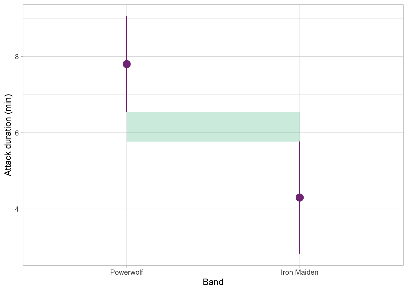
Confidence intervals are typically represented on a plot by “whiskers”, or lines sticking out above and below the mean (which is often represented by a dot or similar small point). The length of the whiskers corresponds to the length of the confidence interval, with the tips of the whiskers ending at the upper and lower bounds of the confidence interval. The “interval” stretches the whole width from the upper to the lower bound, with the mean right in the middle.
The general rule of thumb is this: If the intervals of two groups overlap by less than half of the whisker (half the length of the line going from the point to the end of the interval), then the difference between the two groups will be statistically significant at \(\alpha\) = 0.05. If the overlap is just less than half of the line, then p-value for that comparison will be just less than 0.05. Less overlap will generally be associated with smaller p-value.
Some examples might give you a better idea of how this works.
Here we have a comparison of two groups. The shaded portion of the plot indicates the space between the ends of the confidence intervals. In this case, the confidence intervals don’t overlap at all, so this difference is very likely statistically significant:
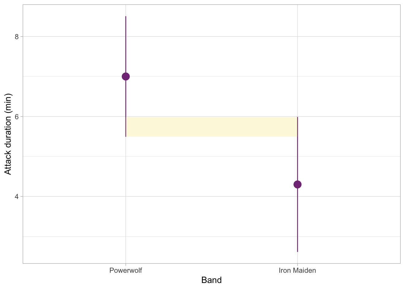
The figure below shows an example with some level of overlap. This time, the shaded portion shows how much the two intervals do overlap. This is still not half of the whisker length, so we can assume that the p-value for this comparison would also be less than 0.05, and therefore the difference could be considered statistically significant.
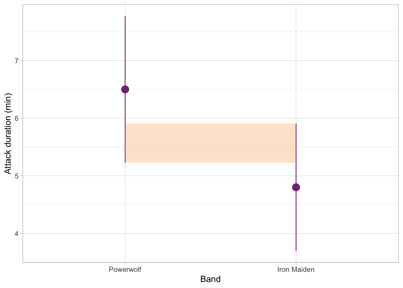
For contrast, the example below is very ambiguous. Eye-balling it, the overlap looks like about a half of each whisker. The p-value would likely hover somewhere around 0.05, either a little bit more or a little bit less.
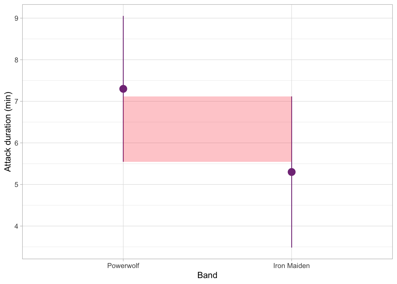
Finally, the figure below shows a situation where the overlap is quite substantial. The difference in orca attack duration between these two groups is unlikely to be statistically significant at 0.05 (in other words, the p-value for this comparison would likely be more than 0.05).
Very well done today! This is the end of the required material for this week. You’ve already learned so much on the module and you’re making great progress.
Not had enough? We love to hear it! Have a go at the ChallengR below.
ChallengR
ChallengR Time!
This task is a ChallengR, which are always optional, and will never be assessed - they’re only there to inspire you to try new things! If you solve this task successfully, you can earn a bonus 2500 Kahoot Points. You can use those points to earn bragging rights and, more importantly, shiny stickers. (See the Games and Awards page on Canvas.)
In order to attempt this week’s ChallengR, you will need to have read through the previous optional section on visually interpreting confidence intervals.
There are no solutions in this document for this ChallengR task. If you get stuck, ask us for help in your practicals or at the Help Desk, and we’ll be happy to point you in the right direction.
To further understand the differences between the effects of Heavy metal and Shrek music on orca attack duration, we might be interested in knowing whether there are differences in durations for different heavy metal bands.
Our dataset contains a variable called band which specifies whether the music that orcas heard was by Iron Maiden, Powerwolf, Opeth, Saor, or Lord of the Lost. That’s quite a few categories, so having all of the summaries for all these groups in a table might get a little overwhelming. So we can create a (gg)plot instead - which will also allow us to visually compare the confidence intervals for these groups.
{ggplot2} Revision
This task requires you to create a plot using the {ggplot2} package. This package was introduced at the end of PAAS, but it’s the first time we’ve used it on this module. If you want a refresher, you might want to look back on weeks 10 and 11 of PAAS and the discovr_05 tutorial on visualising data with {ggplot2}. We will also start creating plots in this module regularly, so this will be excellent practice for the coming weeks!
For this plot, we’re going to look at the mean differences among the categories of the band variable. We’re interested in the differences in mean attack_duration and the respective confidence intervals.
Task 9
Use the orca_tib data to create a plot (using the ggplot2 package) with the attack_duration on the y axis, band on the x axis, with means and confidence intervals for each group.
The plotting function you can use here is stat_summary(fun.data = ????), which will plot the mean and CIs of the groups. Here, the ???? is the same function that we used previously in this tutorial to produce confidence intervals for our table.
Hint
We’re now in {ggplot} territory, so as a reminder, this is what a ggplot code typically looks like:
some_dataset |>
  ggplot2::ggplot(aes(x = variable_for_the_x_axis, y = variable_for_the_y_axis)) +
  plotting_function()
Next
Often the grouping variable goes on the x axis and the continuous/outcome variable goes on the y axis.
Next
The variable band goes on the x axis, and attack_duration goes on the y axis.
Once you have your plot, take the ChallengR quiz on Canvas and use the plot to answer the questions. Good luck, and well done again!
Footnotes
Also known by a more cuddly name - the killer whales.↩︎