library(tidyverse)
library(rempsyc)Skills Lab 09: The linear model (2)
Today’s Session
Plotting a linear model (recap)
Fitting a linear model with one predictor (recap)
Evaluating model fit
Testing hypotheses with linear models
Creating nicely formatted output for reports (if we have time!)
Kahoot!
Tip
Kahoot quizzes are NOT assessed but are great practice for the assessed Canvas quizzes! 😉
Materials
Try out your own solutions in this document
A solutions file will be uploaded to the website after the session.
The Data
Researchers wanted to see whether pet dogs will rescue their owners in a variety of scenarios. They collected information about each dog, including their size, age, sex, and then measured how long it took the dog to rescue their owner who was trapped in a box.
Hypothesis
Dog’s age will be a statistically significant predictor of rescue time.
Load packages and data
Codebook
dog_name- name/id of the dogsex- dog’s sex; coded as 1 for “yes”, 0 for “no”.rescue_time_sec- time (in seconds) it took the dog to rescue their trapped ownervocal_distress_owner- rating of how distressed the owner sounded when calling for help, on a scale 1 (not distressed) to 6 (very distressed)age_months- age of the dog in monthsheight_m- height of the dog in metresweight_kg- height of the dog in kilograms
Task 1: Data cleaning
The age variable is currently recorded in months. For the interpretation, it might be more useful to work with years instead (will be able to tell an increase in rescue time associated with an increase of 1 year)
Create a variable called
age_yearsthat expresses the age in years instead of months.
dog_tib <- dog_tib |>
  dplyr::mutate(
    age_years = age_months/12
  )
Why are we doing this?
Converting to different units is not going to affect any of our statistical tests - it just helps with the interpretation of betas which we’ll eventually get out of the linear model. The betas tell us how the outcome changes with one unit change in the predictor. We’ll see later that it’s easier to think about the result of our model in years, rather than months.
Task 2: Exploring the data
Before fitting any model, it helps to be familiar with your sample.
What’s the average age of the dogs in the sample?
What’s the average rescue time?
Which one of these variables is the outcome and which one is the predictor?
Create a plot showing the relationship between these two variables and interpret it. Do you think this relationship is going to be statistically significant?
dog_tib |>
  dplyr::summarise(
    mean = mean(age_years, na.rm = TRUE),
    sd = sd(age_years, na.rm = TRUE),
  )
# A tibble: 1 × 2
mean sd
<dbl> <dbl>
1 6.09 3.49dog_tib |>
dplyr::summarise(
mean = mean(rescue_time_sec, na.rm = TRUE),
sd = sd(rescue_time_sec, na.rm = TRUE),
)# A tibble: 1 × 2
mean sd
<dbl> <dbl>
1 22.9 27.0Alternatively if you just want to have a quick look and don’t care about whether the information is organised in tables, we could use the summary() function:
dog_tib |>
  dplyr::select(rescue_time_sec, age_years) |>
  summary()
rescue_time_sec age_years
Min. : 0.73 Min. : 1.250
1st Qu.: 5.16 1st Qu.: 2.417
Median : 12.41 Median : 6.583
Mean : 22.85 Mean : 6.088
3rd Qu.: 32.41 3rd Qu.: 8.333
Max. :107.74 Max. :12.000 Let’s create a plot:
dog_tib |>
  ggplot2::ggplot(data = _, aes(x = age_years, y = rescue_time_sec)) +
  geom_point(colour = "darkmagenta") +
  stat_smooth(method = "lm", colour = "darkcyan", fill = "darkcyan", alpha = 0.2) +
  labs(x = "Dog age (years)", y = "Rescue time (sec)") +
  theme_light()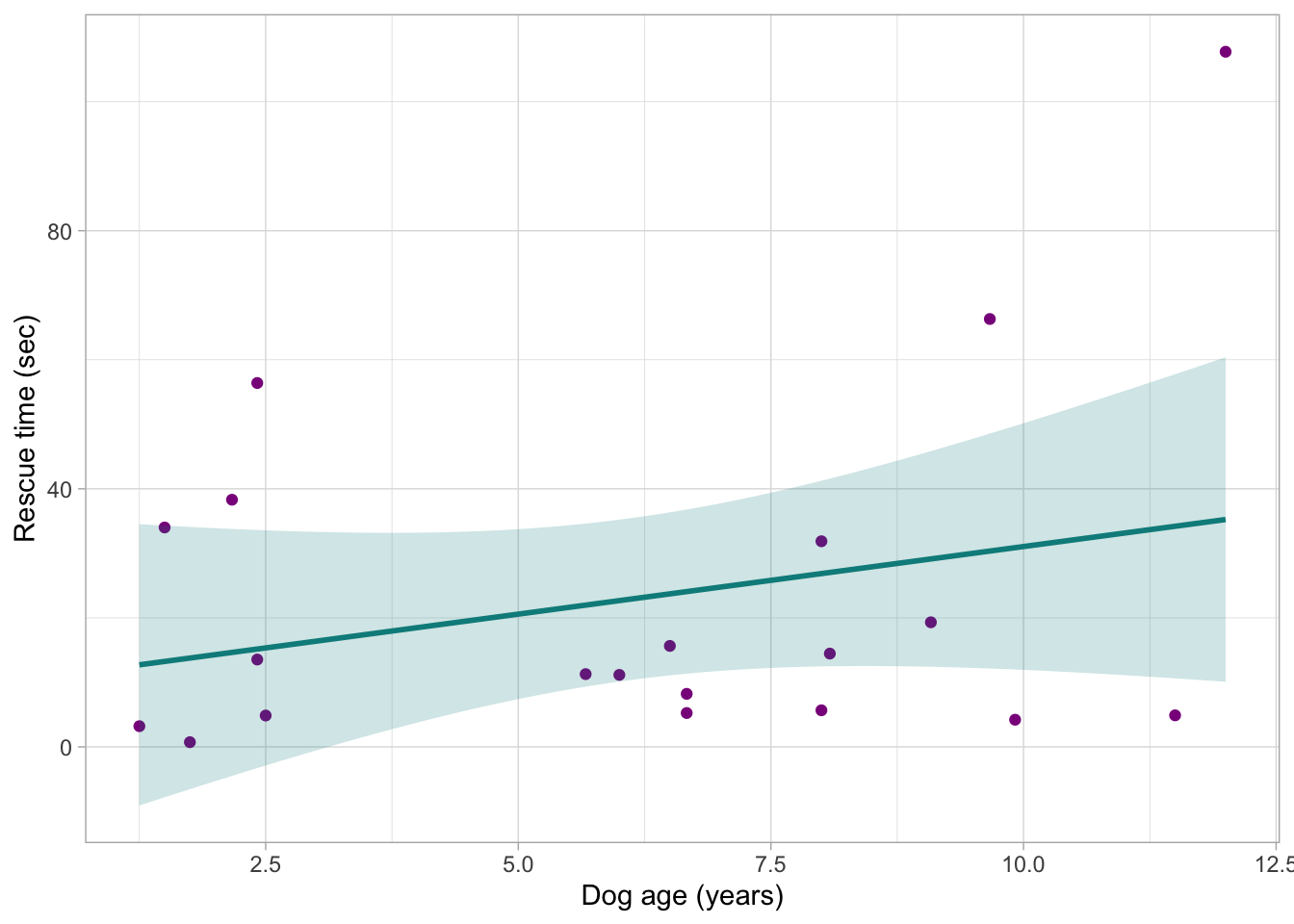
Optional plotting extRas
If you’ve just popped in to check the code for the worksheet, the code above will do the trick. Other stuff to consider we also looked at (because it’s fun):
dog_tib |>
  ggplot2::ggplot(data = _, aes(x = age_years, y = rescue_time_sec, colour = dog_name)) +
  geom_point() +
  stat_smooth(method = "lm", colour = "darkcyan", fill = "darkcyan", alpha = 0.2) +
  labs(x = "Dog age (years)", y = "Rescue time (sec)") +
  theme_light()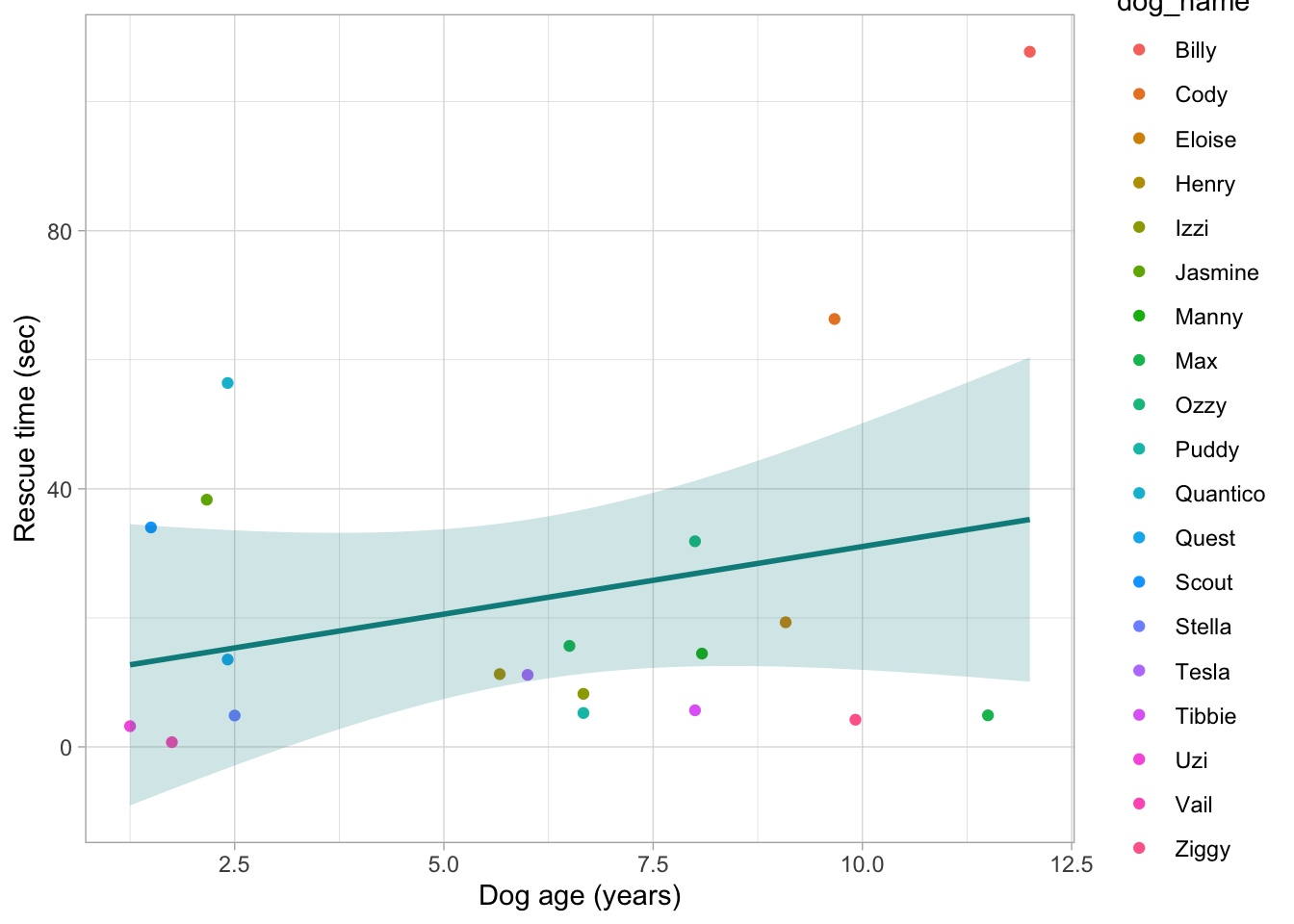
Here I’ve removed the argument colour from geom_point and instead I’ve set the argument colour = dog_name in the aes function in the first line of the plot. When we set the aesthetics instead of setting colour or fill directly in our geom_ or summary_ functions, ggplot will automatically perform any code in ggplot split by the aesthetic we’re specifying. So the colour will be automatically set for each dog name. HOWEVER, if we then specify a colour argument inside of a geom_ function, the aesthetics setting is ignored. This is why the line of best fit isn’t split by different dog names.
When I originally demonstrated this code in the skills lab, it looked like this:
dog_tib |>
  ggplot2::ggplot(data = _, aes(x = age_years, y = rescue_time_sec, colour = dog_name)) +
  geom_point() +
  stat_smooth(method = "lm", alpha = 0.2) +
  labs(x = "Dog age (years)", y = "Rescue time (sec)") +
  theme_light()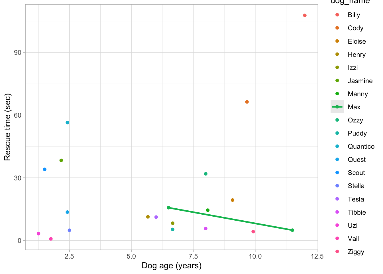
In the code above, I didn’t bother specifying the colour of the line, so ggplot was trying to respect my wishes specified in aes - it wanted to fit the line of best fit for each dog. But we only appear to have a line for Max. How come? Just glancing at the plot, my guess is that there were two dogs called Max. In order to fit a linear model, we need at least two observations. Because Max was the only dog name with two observations, we have a line for Max but no-one else.
Wet paint, do not touch
Generally, we wouldn’t want to show each participant as a separate colour, but there are rare situations when it’s helpful. It’s fine in this scenario, because we only have a handful of dogs.
We certainly wouldn’t want to split colour by subject ID in a dataset that has THOUSANDS of participants, like the smarvus data . Posit cloud might have a bit of a breakdown if we tried, because ggplot would try to represent each participant on a legend, like it did above.
So you know… don’t.
Or do. You’re a scientist, and you’re reading an optional coding session. What’s the worst that could happen? Just save your document before you do so. If you’re feeling like embracing chaos, let Posit cloud crash and then call over a DT or the session lead to see if they can figure out what happen.
-M
Task 3: Fitting the model
The general equation for the linear model is:
\[ y_i = b_0 + b_1x_{1i} + e \]
- What is the equation for our model?
\[ \mbox{Rescue time}_i = b_0 + b_1\mbox{Dog's age}_i + e \]
Fit the model and interpret the intercept and the slope.
Use the
summary()function to obtain the hypothesis test. Can we reject the null hypothesis?
dog_lm <- dog_tib |> lm(rescue_time_sec ~ age_years, data = _)
summary(dog_lm)
Call:
lm(formula = rescue_time_sec ~ age_years, data = dog_tib)

Residuals:
    Min      1Q  Median      3Q     Max
-29.303 -13.741 -10.150   8.948  72.500

Coefficients:
            Estimate Std. Error t value Pr(>|t|)
(Intercept)   10.102     12.237   0.826    0.420
age_years      2.095      1.755   1.194    0.248

Residual standard error: 26.7 on 18 degrees of freedom
Multiple R-squared:  0.07337,   Adjusted R-squared:  0.02189
F-statistic: 1.425 on 1 and 18 DF,  p-value: 0.2481
The \(b_0\) value is 10.102, which means that when the predictor (age) is 0 years, the model predicts a rescue time of only 10.10 seconds (think back to least week about how the intercept is not always a meaningful value in the real world).
The \(b_1\) value is 2.095, rounded to 2.1. This tells us that as age increases by one unit - i.e. with each increase of 1 year - the model predicts an increase of 2 seconds in rescue time.
The p-values are listed in the
Pr(>|t|)column of the output. The p-value forage_yearsis 0.248. This is greater than 0.05, and therefore not statistically significant. We cannot reject the null hypothesis.
Information about the model overall can be found at the bottom the output.
The multiple R2 value is 0.073. This means that the model explains 7.3% of variance. This leaves 92.7% of variance in the model - or the “noise” - unexplained.
The final line tells us about the overall model fit. The non-significant p-value of 0.248 along with the low percentage of variance explained suggests that the model is, on the whole, not a good fit.
Task 4: Nicer looking summaries
When writing reports, we should never present raw R output. We can use the broom package to create nicer summaries.
Use
broom::glance()to extract model fitUse
broom::tidy()to extract info about model coefficients, including confidence intervalsPipe both outputs (individually) into the
rempsyc::nice_table(broom = "lm")function to format it nicely.
dog_lm |>
  broom::glance() |>
  rempsyc::nice_table()
r.squared | adj.r.squared | σ | statistic | p | df | logLik | AIC | BIC | deviance | df.residual | nobs |
|---|---|---|---|---|---|---|---|---|---|---|---|
0.07 | 0.02 | 26.70 | 1.43 | .248 | 1 | -93.02 | 192.03 | 195.02 | 12,830.24 | 18 | 20 |
dog_lm |>
  broom::tidy(conf.int = TRUE) |>
  rempsyc::nice_table()
Term | estimate | std.error | statistic | p | 95% CI |
|---|---|---|---|---|---|
(Intercept) | 10.10 | 12.24 | 0.83 | .420 | [-15.61, 35.81] |
age_years | 2.09 | 1.75 | 1.19 | .248 | [-1.59, 5.78] |
ggpets (optional section)
We also demonstrated how to use the custom custom ggpets package, which is a critical skill for any scientist.
dog_tib |>
  ggplot2::ggplot(data = _, aes(x = age_years, y = rescue_time_sec)) +
  geom_point(colour = "darkmagenta") +
  ggpets::geom_pet(pet = "tibble") +
  stat_smooth(method = "lm", colour = "darkcyan", fill = "darkcyan", alpha = 0.2) +
  labs(x = "Dog age (years)", y = "Rescue time (sec)") +
  theme_light()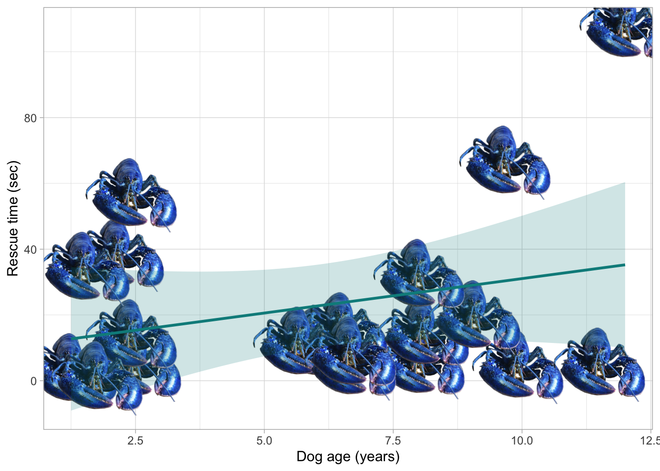
To see all the options for the pet argument, run ?ggpets::geom_pet in the console. This will pull up the help documentation which lists all the pet names. If I accidentally misnamed someone, let me know and I’ll update the package.
-M.