Skills Lab 04: Data Summaries

Author

Data

smarvus_tib <- readr::read_csv("data/smarvus_data.csv")

Codebook

Run this code chunk to open the Codebook in the Viewer tab.

ricomisc::rstudio_viewer("smarvus_codebook.html", "data")

Today’s Task

You are joining an ongoing research project, perhaps on a placement year or for your final-year project. The project is investigating accessibility at University, specifically how diagnosis of specific learning differences (SpLD) impacts students’ experiences. A key research question is whether students with or without diagnosis of SpLD differ in their average levels of adverse experiences, such as anxiety, worry, and fear of being perceived negatively.

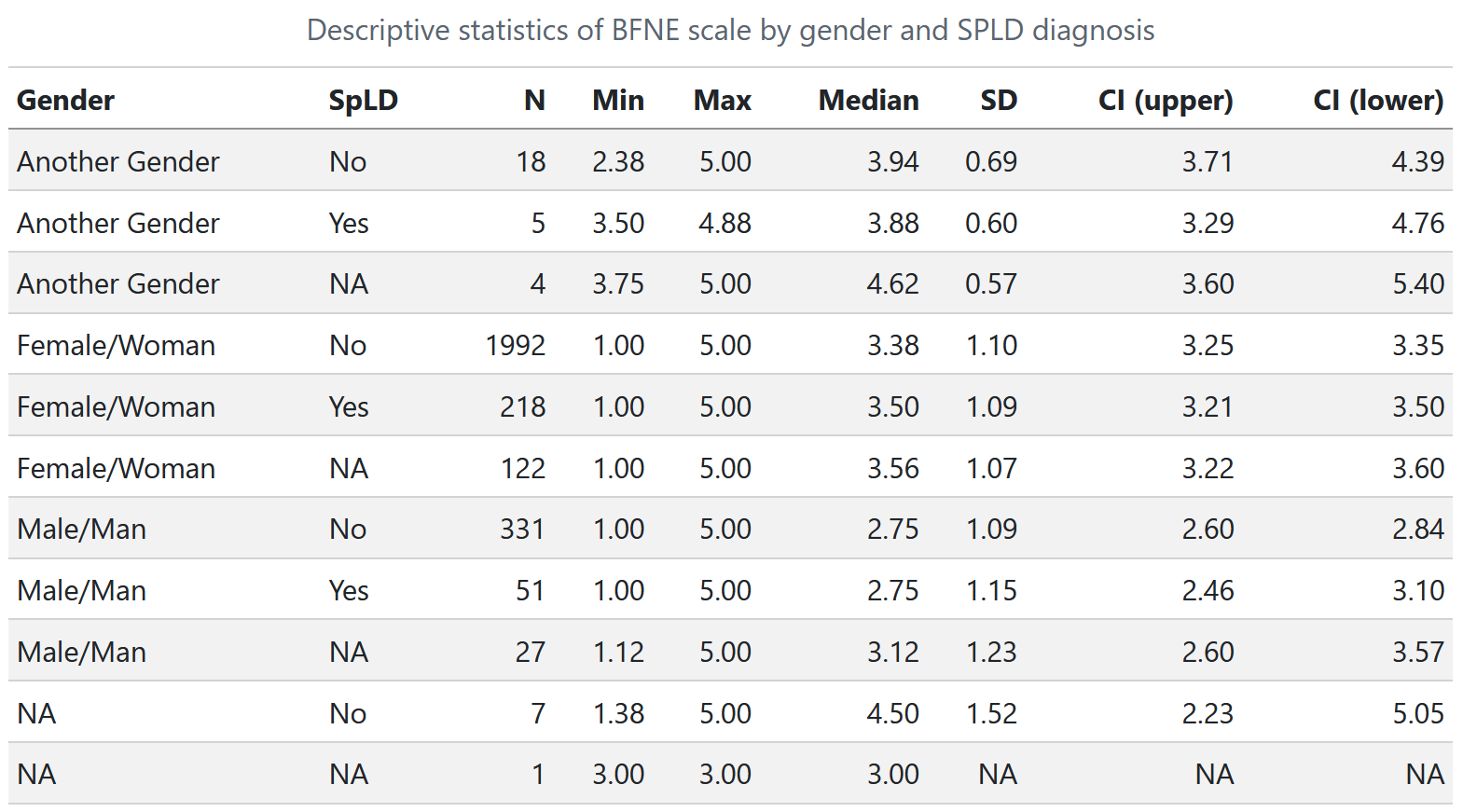
The previous research assistant has already created a summary table of one of the key outcomes, Fear of Negative Evaluation, for the upcoming journal article. Unfortunately, they only included an image of the table, and didn’t save the code to create it! The table looks like this:

Which Measure(s)?

Take a minute to look at this table. What do each of the measures in this table tell us? Why is it useful to calculate and report them? Is there anything important missing that we should include in the table?

Tip

See Tutorial 04 for an explanation!

What To Do?

Our task is to recreate this table, making sure to include all key measures.

Generic Summaries

First, we can easily get some overall information about our numeric variables with some useful functions.

summary(smarvus_tib)

datawizard::describe_distribution(smarvus_tib)

Consider This:

What is useful about the output from these summary functions? What can we use them for?

What can we NOT (easily) use them for?

Solution

This is a great way for you, the analyst, to get a quick look at the data. Without having to do any extra coding, you have useful overall information about most or all of the variables in your dataset. This lets you easily spot problems and get a sense of your data.

However, there are two main issues. First, we can’t very easily see or control what is included in this output. Both summary() and describe_distribution() have some arguments we can change (see the help documentation), but not everything, and it isn’t obvious how to do this.

Second, this is not a great way to present this information. This output isn’t nicely formatted; it would not be a good way to include this summary info in a report.

So, we should make our own summaries instead, that include the information we want, and that look nice in our reports (or take-away papers 👀).

Summarising A Variable

First, let’s calculate summary statistics for the outcome variable, bfne, using dplyr::summarise().

smarvus_tib |> 
  dplyr::summarise(
    n = dplyr::n(), 
    min = min(bfne, na.rm = TRUE), 
    max = max(bfne, na.rm = TRUE), 
    ## Mean wasn't in the original table, but is a crucial element for the research question
    mean = mean(bfne, na.rm = TRUE), 
    median = median(bfne, na.rm = TRUE), 
    sd = sd(bfne, na.rm = TRUE), 
    ci_lower = ggplot2::mean_cl_normal(bfne)$ymin,
    ci_upper = ggplot2::mean_cl_normal(bfne)$ymax
  )

# A tibble: 1 × 8
      n   min   max  mean median    sd ci_lower ci_upper
  <int> <dbl> <dbl> <dbl>  <dbl> <dbl>    <dbl>    <dbl>
1  2776     1     5  3.24   3.38  1.12     3.20     3.28

Consider This: CIs vs SDs

Why is it that this variable has a relatively large SD (compared to the scale it’s measured on), but an extremely narrow CI?

Solution

Remember that CIs are calculated based on the square root of the sample size - and that’s quite big here!

Consider This: Returning NAs

Why is it that functions like mean and median return NA if they have even one missing value?

Tip

See Tutorial 04 for an explanation!

Summarising by Groups

Next, we want to split our summary table into different rows, one for each category in two predictors: gender and spld.

First, what happens when we group_by() a variable?

smarvus_tib |>
  dplyr::group_by(spld)

# A tibble: 2,776 × 34
# Groups:   spld [3]
   unique_id country   language university degree_major degree_year age   gender
   <chr>     <chr>     <chr>    <chr>      <chr>        <chr>       <chr> <chr> 
 1 X8V0T6    Netherla… English  Universit… Psychology   1st Year    18-21 Femal…
 2 J3W3Y7    England   English  Universit… Psychology   1st Year    18-21 Femal…
 3 S7C2L2    England   English  Universit… Psychology   1st Year    22-25 Femal…
 4 Y4Z6A6    Scotland  English  Universit… Psychology   1st Year    26+   Femal…
 5 L2O9Z1    Australia English  Macquarie… Psychology   1st Year    18-21 Femal…
 6 B5I6O0    Austria   German   Universit… Psychology   1st Year    18-21 Femal…
 7 N8H9D1    England   English  Loughboro… Psychology   1st Year    18-21 Male/…
 8 F2J7V4    England   English  Bournemou… Psychology   1st Year    18-21 Femal…
 9 N9M3V8    Germany   German   Universit… Psychology   1st Year    18-21 Femal…
10 O3F8F8    Australia English  Macquarie… Psychology   1st Year    18-21 Femal…
# ℹ 2,766 more rows
# ℹ 26 more variables: spld <chr>, in_person_lectures <chr>,
#   in_person_practicals <chr>, atms_per <dbl>, belief <dbl>, bfne <dbl>,
#   cas_cre <dbl>, cas_non <dbl>, crt <dbl>, ius_sf_inh <dbl>,
#   ius_sf_pro <dbl>, lsas_sr_per <dbl>, lsas_sr_soc <dbl>, ngse <dbl>,
#   r_mars_course <dbl>, r_mars_num <dbl>, r_mars_test <dbl>, r_tas_bod <dbl>,
#   r_tas_ten <dbl>, r_tas_tes <dbl>, r_tas_worry <dbl>, stars_ask <dbl>, …

Notice the Groups: spld [3] at the top of our tibble. This means that our tibble is grouped by the values of our spld variable, so any subsequent calculations will take place inside those groups. Let’s see what that might look like.

## SAME code as above, just with the new group_by line!

smarvus_tib |> 
  dplyr::group_by(spld) |> ## Only this is added
  dplyr::summarise(
    n = dplyr::n(), 
    min = min(bfne, na.rm = TRUE), 
    max = max(bfne, na.rm = TRUE), 
    mean = mean(bfne, na.rm = TRUE), 
    median = median(bfne, na.rm = TRUE), 
    sd = sd(bfne, na.rm = TRUE), 
    ci_lower = ggplot2::mean_cl_normal(bfne)$ymin,
    ci_upper = ggplot2::mean_cl_normal(bfne)$ymax
  )

# A tibble: 3 × 9
  spld      n   min   max  mean median    sd ci_lower ci_upper
  <chr> <int> <dbl> <dbl> <dbl>  <dbl> <dbl>    <dbl>    <dbl>
1 No     2348     1     5  3.23   3.25  1.12     3.18     3.27
2 Yes     274     1     5  3.26   3.38  1.12     3.13     3.39
3 <NA>    154     1     5  3.38   3.56  1.10     3.20     3.56

So, we get the same information as we did before, but now it’s split up by the groups in the spld variable.

Summarising by Multiple Groups

What do you think will happen when we add in a second categorical variable?

## SAME code as above, now with two categorical variables in group_by

smarvus_tib |> 
  dplyr::group_by(gender, spld) |> 
  dplyr::summarise(
    n = dplyr::n(), 
    min = min(bfne, na.rm = TRUE), 
    max = max(bfne, na.rm = TRUE), 
    mean = mean(bfne, na.rm = TRUE), 
    median = median(bfne, na.rm = TRUE), 
    sd = sd(bfne, na.rm = TRUE), 
    ci_lower = ggplot2::mean_cl_normal(bfne)$ymin,
    ci_upper = ggplot2::mean_cl_normal(bfne)$ymax
  )

# A tibble: 11 × 10
# Groups:   gender [4]
   gender         spld      n   min   max  mean median     sd ci_lower ci_upper
   <chr>          <chr> <int> <dbl> <dbl> <dbl>  <dbl>  <dbl>    <dbl>    <dbl>
 1 Another Gender No       18  2.38  5     4.05   3.94  0.688     3.71     4.39
 2 Another Gender Yes       5  3.5   4.88  4.03   3.88  0.596     3.29     4.76
 3 Another Gender <NA>      4  3.75  5     4.5    4.62  0.568     3.60     5.40
 4 Female/Woman   No     1992  1     5     3.30   3.38  1.10      3.25     3.35
 5 Female/Woman   Yes     218  1     5     3.35   3.5   1.09      3.21     3.50
 6 Female/Woman   <NA>    122  1     5     3.41   3.56  1.07      3.22     3.60
 7 Male/Man       No      331  1     5     2.72   2.75  1.09      2.60     2.84
 8 Male/Man       Yes      51  1     5     2.78   2.75  1.15      2.46     3.10
 9 Male/Man       <NA>     27  1.12  5     3.08   3.12  1.23      2.60     3.57
10 <NA>           No        7  1.38  5     3.64   4.5   1.52      2.23     5.05
11 <NA>           <NA>      1  3     3     3      3    NA        NA       NA

Making Pretty HTML Tables

Recall some of the issues we identified previously with summary functions (like summary())

We can’t very easily see or control what is included in this output.
This output isn’t nicely formatted and it would not be a good way to include this summary info in a report.

We’ve resolved (1) by choosing what appears in the output, but this is still just a tibble and pretty ugly! The knitr::kable() function is the basic tool to turn tibbles into nicely formatted, report-worthy HTML tables. Let’s have a look:

smarvus_tib |> 
  dplyr::group_by(gender, spld) |> 
  dplyr::summarise(
    n = dplyr::n(), 
    min = min(bfne, na.rm = TRUE), 
    max = max(bfne, na.rm = TRUE), 
    mean = mean(bfne, na.rm = TRUE), 
    median = median(bfne, na.rm = TRUE), 
    sd = sd(bfne, na.rm = TRUE), 
    ci_lower = ggplot2::mean_cl_normal(bfne)$ymin,
    ci_upper = ggplot2::mean_cl_normal(bfne)$ymax
  ) |> 
  ## Same code as above up to here
  knitr::kable(
    ## Give a list of names in c() to rename the columns
    ## Use nicely formatted real words, NOT variable names!
    col.names = c("Gender", "SpLD", "N", "Min", "Max", "Mean", "Median", "SD", "CI~upper~", "CI~lower~"),
    ## Round number of decimal places
    digits = 2,
    ## Add a caption
    caption = "Descriptive statistics of BFNE scale by gender and SPLD diagnosis",
  ) |> 
  kableExtra::kable_styling()

Descriptive statistics of BFNE scale by gender and SPLD diagnosis
Gender	SpLD	N	Min	Max	Mean	Median	SD	CI~upper~	CI~lower~
Another Gender	No	18	2.38	5.00	4.05	3.94	0.69	3.71	4.39
Another Gender	Yes	5	3.50	4.88	4.03	3.88	0.60	3.29	4.76
Another Gender	NA	4	3.75	5.00	4.50	4.62	0.57	3.60	5.40
Female/Woman	No	1992	1.00	5.00	3.30	3.38	1.10	3.25	3.35
Female/Woman	Yes	218	1.00	5.00	3.35	3.50	1.09	3.21	3.50
Female/Woman	NA	122	1.00	5.00	3.41	3.56	1.07	3.22	3.60
Male/Man	No	331	1.00	5.00	2.72	2.75	1.09	2.60	2.84
Male/Man	Yes	51	1.00	5.00	2.78	2.75	1.15	2.46	3.10
Male/Man	NA	27	1.12	5.00	3.08	3.12	1.23	2.60	3.57
NA	No	7	1.38	5.00	3.64	4.50	1.52	2.23	5.05
NA	NA	1	3.00	3.00	3.00	3.00	NA	NA	NA

Looking good!

New Functions: knitr::kable() and kableExtra::kable_styling()

The kable() + kable_styling() tag team has a lot of options to make your tables look very pretty in HTML format (which is what we typically render to, including on the TAP 👀). You can put any tibble into kable() and use it to add nice formatting to the output, so rendered HTML documents - like take-away papers 👀 👀 👀 - present your results in a professional way.

Today we’ve looked at three main arguments in kable() to get you started:

col.names will take a vector of names that it will use for the column names in your table. Be careful to check that the names you put in match with your data!
digits takes a single number, and will round any numbers to that number of decimal places.
caption takes a string, and outputs a nicely formatted caption.

kable_styling() can be customised further, but it does a lot of the heavy lifting without any extra input.

Tip

Want more kable()? Check out the indispensable Create Awesome HTML Tables documentation if you really want to jazz up your tables.

Render

Let’s try and render the document… 🤞

Data

Codebook

Today’s Task

Which Measure(s)?

What To Do?

Generic Summaries

Summarising A Variable

Summarising by Groups

Summarising by Multiple Groups

Making Pretty HTML Tables

Render

Kahoot time!